Hidden Markov Model (HMM) in NLP: Complete Implementation in Python

In the previous article, we discussed Lexicon and the rule-based POS tagging approach and also did the implementation in Python. In this article, we will discuss the Hidden Markov model in detail which is one of the probabilistic (stochastic) POS tagging methods. Further, we will also discuss Markovian assumptions on which it is based, its applications, advantages, and limitations along with its complete implementation in Python.

Natural Language Processing (NLP) is a rapidly growing field that aims to teach machines to understand and interpret human language. One of the most important tools in NLP is the Hidden Markov Model (HMM).

The Hidden Markov Model is a statistical model that is used to analyze sequential data, such as language, and is particularly useful for tasks like speech recognition, machine translation, and text analysis.

But before deep diving into Hidden Markov Model, we first need to understand the Markovian assumption.

Markovian Assumption

Markov models are stochastic models that were created to model processes that occur sequentially. In a Markov process, it is typically assumed that the probability of each event or state depends only on the probability of the preceding event. This simplifying assumption is known as the Markovian assumption, and it is a special case of a one-Markov or first-order Markov assumption.

Markov Chain

A Markov chain is a mathematical model that represents a process where the system transitions from one state to another. The transition assumes that the probability of moving to the next state is solely dependent on the current state. Please refer to the figure below for an illustration:

In the above figure, ‘a’, ‘p’, ‘i’, ‘t’, ‘e’, and ‘h’ represent the states, while the numbers on the edges indicate the probability of transitioning from one state to another. For example, the probability of transitioning from state ‘t’ to states ‘i’, ‘a’, and ‘h’ are 0.3, 0.3, and 0.4, respectively.

The start state is a special state that represents the initial state of the process, such as the start of a sentence.

Markov processes are commonly used to model sequential data, like text and speech.

For instance, if you want to build an application that predicts the next word in a sentence, you can represent each word in a sentence as a state. The transition probabilities can be learned from a corpus and represent the probability of moving from the current word to the next word.

For example, the transition probability from the state ‘San’ to ‘Francisco’ will be higher than the probability of transitioning to the state ‘Delhi’.

Hidden Markov Model

The Hidden Markov Model (HMM) is an extension of the Markov process used to model phenomena where the states are hidden or latent, but they emit observations. For instance, in a speech recognition system like a speech-to-text converter, the states represent the actual text words to predict, but they are not directly observable (i.e., the states are hidden). Rather, you only observe the speech (audio) signals corresponding to each word and need to deduce the states using the observations.

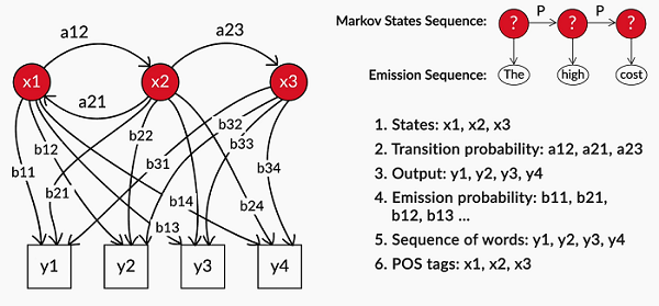
Similarly, in POS tagging, you observe the words in a sentence, but the POS tags themselves are hidden. Thus, the POS tagging task can be modeled as a Hidden Markov Model with the hidden states representing POS tags that emit observations, i.e., words.

The hidden states emit observations with a certain probability. Therefore, Hidden Markov Model has emission probabilities, which represent the probability that a particular state emits a given observation. Along with the transition and initial state probabilities, these emission probabilities are used to model HMMs.

The figure below illustrates the emission and transition probabilities for a hidden Markov process with three hidden states and four observations.

HMM can be trained using a variety of algorithms, including the Baum-Welch algorithm and the Viterbi algorithm.

The Baum-Welch algorithm is an unsupervised learning algorithm that iteratively adjusts the probabilities of events occurring in each state to fit the data better.

The Viterbi algorithm is a dynamic programming algorithm that finds the most likely sequence of hidden states given a sequence of observable events.

Viterbi Algorithm

The Viterbi algorithm is a dynamic programming algorithm used to determine the most probable sequence of hidden states in a Hidden Markov Model (HMM) based on a sequence of observations. It is a widely used algorithm in speech recognition, natural language processing, and other areas that involve sequential data.

The algorithm works by recursively computing the probability of the most likely sequence of hidden states that ends in each state for each observation.

At each time step, the algorithm computes the probability of being in each state and emits the current observation based on the probabilities of being in the previous states and making a transition to the current state.

Assuming we have an HMM with N hidden states and T observations, the Viterbi algorithm can be summarized as follows:

1. Initialization: At time t=1, we set the probability of the most likely path ending in state i for each state i to the product of the initial state probability pi and the emission probability of the first observation given state i. This is denoted by: delta[1,i] = pi * b[i,1].
2. Recursion: For each time step t from 2 to T, and for each state i, we compute the probability of the most likely path ending in state i at time t by considering all possible paths that could have led to state i. This probability is given by:

delta[t,i] = max_j(delta[t-1,j] * a[j,i] * b[i,t])

Here, a[j,i] is the probability of transitioning from state j to state i, and b[i,t] is the probability of observing the t-th observation given state I.

We also keep track of the most likely previous state that led to the current state i, which is given by:

psi[t,i] = argmax_j(delta[t-1,j] * a[j,i])

3. Termination: The probability of the most likely path overall is given by the maximum of the probabilities of the most likely paths ending in each state at time T. That is, P* = max_i(delta[T,i]).
4. Backtracking: Starting from the state i* that gave the maximum probability at time T, we recursively follow the psi values back to time t=1 to obtain the most likely path of hidden states.

The Viterbi algorithm is an efficient and powerful tool that can handle long sequences of observations using dynamic programming.

Advantages of the Hidden Markov Model

One of the advantages of HMM is its ability to learn from data.

HMM can be trained on large datasets to learn the probabilities of certain events occurring in certain states.

For example, HMM can be trained on a corpus of sentences to learn the probability of a verb following a noun or an adjective.

Applications of the Hidden Markov Model

• Part-of-Speech (POS) Tagging
• Named Entity Recognition (NER)
• Speech Recognition
• Machine Translation

Limitations of the Hidden Markov Model

HMM assumes that the probability of an event occurring in a certain state is fixed, which may not always be the case in real-world data. Additionally, HMM is not well-suited for modeling long-term dependencies in language, as it only considers the immediate past.

There are alternative models to HMM in NLP, including recurrent neural networks (RNNs) and transformer models like BERT and GPT. These models have shown promising results in a variety of NLP tasks, but they also have their own limitations and challenges.

Implementation of the Hidden Markov Model in Python

In this Python implementation of HMM, we will try to code the Viterbi heuristic using the tagged Treebank corpus.

Exploring Treebank Tagged Corpus

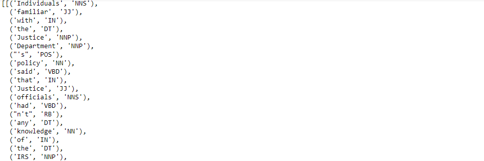
#Importing libraries
import nltk, re, pprint
import numpy as np
import pandas as pd
import requests
import matplotlib.pyplot as plt
import seaborn as sns
import pprint, time
import random
from sklearn.model_selection import train_test_split
from nltk.tokenize import word_tokenize

# reading the Treebank tagged sentences
wsj = list(nltk.corpus.treebank.tagged_sents())

# first few tagged sentences
print(wsj[:40])

As we can observe from the above output, each word in the sentence is tagged with its corresponding POS tag.

Train Test Split

In this step, we will split the dataset into a 70:30 ratio i.e., 70% of the data for the training set and the rest 30% for the test set.

# Splitting into train and test
random.seed(1234)
train_set, test_set = train_test_split(wsj,test_size=0.3)

print(len(train_set))
print(len(test_set))
print(train_set[:40])

From the above output, we can observe that the total number of training records is 2739, and the test set has 1175. The top 40 sentences are also shown in which each word is tagged to its POS tag.

Next, we will check the number of tagged words in the training set to understand how much data will be used for training the POS tagger.

# Getting list of tagged words
train_tagged_words = [tup for sent in train_set for tup in sent]
len(train_tagged_words)

Output

70503

Next, we will create a tokens variable that will contain all the tokens from the train_tagged_words. Furthermore, we also need to create a vocabulary and set of all unique tags in the training data.

# tokens 
tokens = [pair[0] for pair in train_tagged_words]
# vocabulary
V = set(tokens)
print("Total vocabularies: ",len(V))
# number of tags
T = set([pair[1] for pair in train_tagged_words])
print("Total tags: ",len(T))

Output

Total vocabularies: 10236
Total tags: 46

Next, we will use HMM algorithm to tag the words.

Given a sequence of words to be tagged, the task is to assign the most probable tag to the word.

In other words, to every word w, assign the tag t that maximizes the likelihood P(t/w). Since P(t/w) = P(w/t). P(t) / P(w), after ignoring P(w), we have to compute P(w/t) and P(t).

P(w/t) is basically the probability that given a tag (say NN), what is the probability of it being w (say ‘building’). This can be computed by computing the fraction of all NNs which are equal to w, i.e.

P(w/t) = count(w, t) / count(t).

The term P(t) is the probability of tag t, and in a tagging task, we assume that a tag will depend only on the previous tag. In other words, the probability of a tag being NN will depend only on the previous tag t(n-1). So for e.g. if t(n-1) is a JJ, then t(n) is likely to be an NN since adjectives often precede a noun (blue coat, tall building, etc.).

Given the Penn treebank tagged dataset, we can compute the two terms P(w/t) and P(t) and store them in two large matrices. The matrix of P(w/t) will be sparse since each word will not be seen with most tags ever, and those terms will thus be zero.

Emission probabilities

# computing P(w/t) and storing in T x V matrix
t = len(T)
v = len(V)
w_given_t = np.zeros((t, v))

# compute word given tag: Emission Probability
def word_given_tag(word, tag, train_bag = train_tagged_words):
    tag_list = [pair for pair in train_bag if pair[1]==tag]
    count_tag = len(tag_list)
    w_given_tag_list = [pair[0] for pair in tag_list if pair[0]==word]
    count_w_given_tag = len(w_given_tag_list)
    
    return (count_w_given_tag, count_tag)

# examples

# large
print("\n", "large")
print(word_given_tag('large', 'JJ'))
print(word_given_tag('large', 'VB'))
print(word_given_tag('large', 'NN'), "\n")

# will
print("\n", "will")
print(word_given_tag('will', 'MD'))
print(word_given_tag('will', 'NN'))
print(word_given_tag('will', 'VB'))

# book
print("\n", "book")
print(word_given_tag('book', 'NN'))
print(word_given_tag('book', 'VB'))

Transition Probabilities

# compute tag given tag: tag2(t2) given tag1 (t1), i.e. Transition Probability

def t2_given_t1(t2, t1, train_bag = train_tagged_words):
    tags = [pair[1] for pair in train_bag]
    count_t1 = len([t for t in tags if t==t1])
    count_t2_t1 = 0
    for index in range(len(tags)-1):
        if tags[index]==t1 and tags[index+1] == t2:
            count_t2_t1 += 1
    return (count_t2_t1, count_t1)

# examples
print(t2_given_t1(t2='NNP', t1='JJ'))
print(t2_given_t1('NN', 'JJ'))
print(t2_given_t1('NN', 'DT'))
print(t2_given_t1('NNP', 'VB'))
print(t2_given_t1(',', 'NNP'))
print(t2_given_t1('PRP', 'PRP'))
print(t2_given_t1('VBG', 'NNP'))

#Please note P(tag|start) is same as P(tag|'.')
print(t2_given_t1('DT', '.'))
print(t2_given_t1('VBG', '.'))
print(t2_given_t1('NN', '.'))
print(t2_given_t1('NNP', '.'))

Next, we will create a transition matrix of tags of dimension txt

# creating t x t transition matrix of tags
# each column is t2, each row is t1
# thus M(i, j) represents P(tj given ti)

tags_matrix = np.zeros((len(T), len(T)), dtype='float32')
for i, t1 in enumerate(list(T)):
    for j, t2 in enumerate(list(T)): 
        tags_matrix[i, j] = t2_given_t1(t2, t1)[0]/t2_given_t1(t2, t1)[1]

tags_matrix

As tags are not visible in this matrix, we will now convert it into pandas dataframe for better readability.

# convert the matrix to a df for better readability
tags_df = pd.DataFrame(tags_matrix, columns = list(T), index=list(T))
tags_df

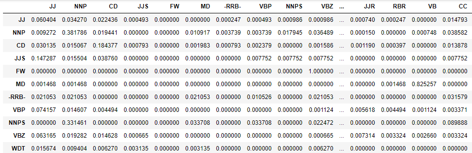
Next will create a heatmap of the tag matrix

# heatmap of tags matrix
# T(i, j) means P(tag j given tag i)
plt.figure(figsize=(18, 12))
sns.heatmap(tags_df)
plt.show()

Now, in order to see the most frequent tags we have to filter the tags with >0.5 probability

# frequent tags
# filter the df to get P(t2, t1) > 0.5
tags_frequent = tags_df[tags_df>0.5]
plt.figure(figsize=(18, 12))
sns.heatmap(tags_frequent)
plt.show()

Next, we will use the Viterbi algorithm

Viterbi Algorithm

Let’s now use the computed probabilities P(w, tag) and P(t2, t1) to assign tags to each word in the document. We’ll run through each word w and compute P(tag/w)=P(w/tag).P(tag) for each tag in the tag set, and then assign the tag having the max P(tag/w).

We’ll store the assigned tags in a list of tuples, similar to the list ‘train_tagged_words’. Each tuple will be a (token, assigned_tag). As we progress further in the list, each tag to be assigned will use the tag of the previous token.

Note: P(tag|start) = P(tag|’.’)

# Viterbi Heuristic
def Viterbi(words, train_bag = train_tagged_words):
    state = []
    T = list(set([pair[1] for pair in train_bag]))
    
    for key, word in enumerate(words):
        #initialise list of probability column for a given observation
        p = [] 
        for tag in T:
            if key == 0:
                transition_p = tags_df.loc['.', tag]
            else:
                transition_p = tags_df.loc[state[-1], tag]
                
            # compute emission and state probabilities
            emission_p = word_given_tag(words[key], tag)[0]/word_given_tag(words[key], tag)[1]
            state_probability = emission_p * transition_p    
            p.append(state_probability)
            
        pmax = max(p)
        # getting state for which probability is maximum
        state_max = T[p.index(pmax)] 
        state.append(state_max)
    return list(zip(words, state))

Evaluating on Test Set

# Running on entire test dataset would take more than 3-4hrs. 
# Let's test our Viterbi algorithm on a few sample sentences of test dataset

random.seed(1234)

# choose random 5 sents
rndom = [random.randint(1,len(test_set)) for x in range(5)]

# list of sents
test_run = [test_set[i] for i in rndom]

# list of tagged words
test_run_base = [tup for sent in test_run for tup in sent]

# list of untagged words
test_tagged_words = [tup[0] for sent in test_run for tup in sent]
test_run

now, we will tag the test sentences using the Viterbi algorithm

# tagging the test sentences
start = time.time()
tagged_seq = Viterbi(test_tagged_words)
end = time.time()
difference = end-start
print("Time taken in seconds: ", difference)
print(tagged_seq)

As we can see it has taken around 122 seconds and it has tagged all the words in the test sentences. Now in order to check the accuracy we have to execute the below code.

# accuracy
check = [i for i, j in zip(tagged_seq, test_run_base) if i == j] 
accuracy = len(check)/len(tagged_seq)
print(accuracy)

Output

0.8736263736263736

Our POS tagger model, which is based on HMM, achieves a reasonably good accuracy of 87.36% for POS tagging.

Now let’s test the model on a sample sentence.

## Testing
sentence_test = 'Twitter is the best networking social site. Man is a social animal. Data science is an emerging field. Data science jobs are high in demand.'
words = word_tokenize(sentence_test)

start = time.time()
tagged_seq = Viterbi(words)
print(tagged_seq)

As we can see HMM model has done a reasonably good job of tagging a sample sentence.

Conclusion

In this article, we have covered a comprehensive discussion on HMM, including its Markovian assumption, limitations, advantages, and applications. We have also explored the Viterbi algorithm for HMM and demonstrated its implementation using Python.