
Table of Contents
Breast cancer is now the most commonly diagnosed cancer in women worldwide, overtaking lung cancer, according to statistics released by the International Agency for Research on Cancer (IARC) in December 2020.
The overall number of people diagnosed with cancer has nearly doubled in the last two decades, from an estimated 10 million in 2000 to 19.3 million in 2020.
The projected trend indicates that the number of cancer cases will increase further in the coming years and will be nearly 50% higher in 2040 than in 2020.

In this article, we have demonstrated how we can perform breast cancer prediction using a machine learning algorithm support vector machine for predicting if the breast cancer diagnosis is benign or malignant.
Understanding Dataset
In this project, we have used Breast Cancer Wisconsin (Diagnostic) Data Set available in UCI Machine Learning Repository for building a breast cancer prediction model. The dataset comprises 569 instances, with a class distribution of 357 benign and 212 malignant cases. Each sample includes an ID number, a diagnosis of either benign (B) or malignant (M), and 30 features.
These features have been computed from a digitized image of a fine needle aspirate (FNA) of a breast mass. For each cell nucleus, ten real-valued features (as listed in the table below) were calculated.
| S.No. | Feature | Description |
| 1. | Radius | mean of distances from the center to points on the perimeter |
| 2. | Texture | standard deviation of grey-scale values |
| 3. | Perimeter | |
| 4. | Area | |
| 5. | Smoothness | local variation in radius lengths |
| 6. | Compactness | (perimeter^2/area – 1.0) |
| 7. | Concavity | severity of concave portions of the contour |
| 8. | Concave points | number of concave portions of the contour |
| 9. | Symmetry | |
| 10. | Fractal dimension | “coastline approximation” − 1 |
The mean, standard error, and the “worst” or largest (mean of the three largest values) of these features were then computed for each image, resulting in a total of 30 features.
Let’s look into the actual snapshot of the dataset by reading the data using the pandas library.
# import libraries
import pandas as pd # Import Pandas for data manipulation using dataframes
import numpy as np # Import Numpy for data statistical analysis
import matplotlib.pyplot as plt # Import matplotlib for data visualisation
import seaborn as sns # Statistical data visualization
# %matplotlib inline

# Import Cancer data drom the Sklearn library
from sklearn.datasets import load_breast_cancer
cancer = load_breast_cancer()

cancer
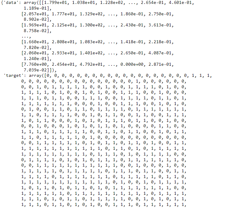
As we can observe data is available in very raw form in dictionary format. So we have to convert it into pandas dataframe format.
df_cancer = pd.DataFrame(np.c_[cancer['data'], cancer['target']], columns = np.append(cancer['feature_names'], ['target']))
df_cancer.head()
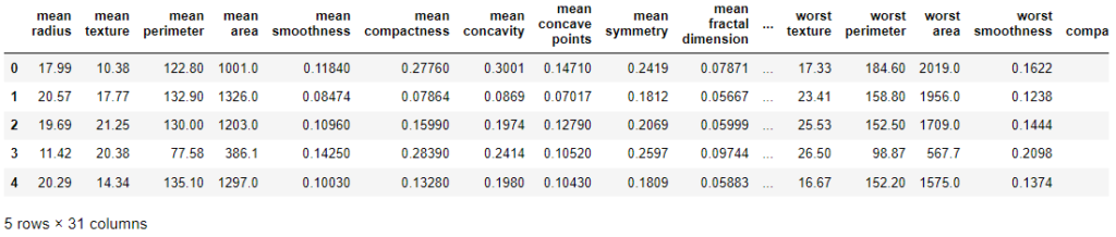
So, we have successfully converted the data into data frame format.
Now, next, we will visualize the data to understand the underlying pattern in the dataset.
Exploratory Data Analysis
First, we will visualize the main mean features using Seaborn library pairplot.
sns.pairplot(df_cancer, hue = 'target', vars = ['mean radius', 'mean texture', 'mean area', 'mean perimeter', 'mean smoothness']
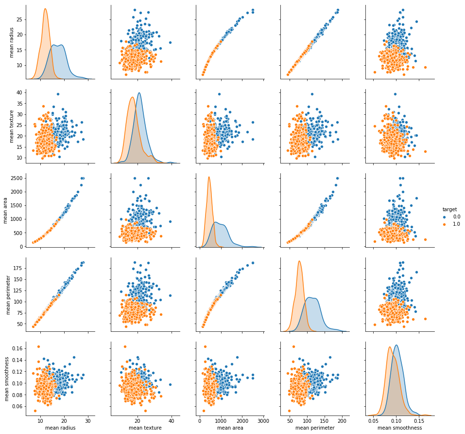
From the above visualization, we can observe that all the features i.e., mean radius, mean perimeter, mean texture, and mean smoothness for malignant cases (i.e., target=0) are higher than benign cases.
Next, we will check the distribution of the target variable to detect whether the data is balanced or imbalanced.
sns.countplot(df_cancer['target'], label = "Count")
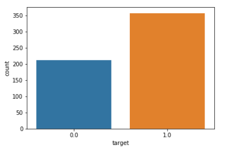
From the above plot, it is clear that malignant cases are around 200 whereas benign have the majority with approx 350 cases.
Next, we will check the mean_area and mean_smoothness feature plots to understand their relationship.
sns.scatterplot(x = 'mean area', y = 'mean smoothness', hue = 'target', data = df_cancer)
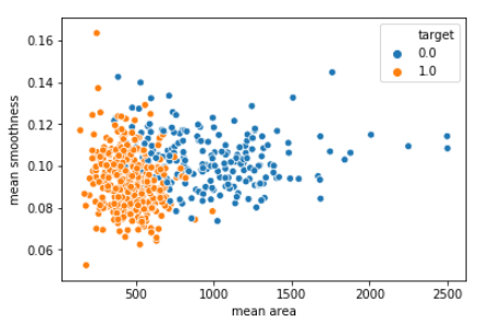
As per the plot, we can observe that with lower mean_smoothness and higher mean_area malignant cases are higher than benign cases.
Next, we will plot a correlation matrix to understand the dependencies of the features among them.
# Let's check the correlation between the variables
# Strong correlation between the mean radius and mean perimeter, mean area and mean primeter
plt.figure(figsize=(20,10))
sns.heatmap(df_cancer.corr(), annot=True)
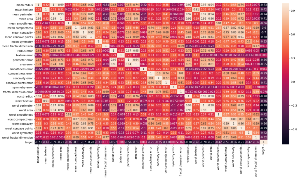
As from the plot, it is evident that worst_perimeter and worst_area are highly correlated with mean_area and mean_perimeter.
Model Training
For building the machine learning model, first, we have to segregate feature and target variables.
# Let's drop the target label coloumns
X = df_cancer.drop(['target'],axis=1)
y = df_cancer['target']
Next, we will do Train Test splitting by taking 80% of the data for training the model and rest for testing the model.
from sklearn.model_selection import train_test_split

X_train, X_test, y_train, y_test = train_test_split(X, y, test_size = 0.20, random_state=5)
as we have segregated the data, now we have to build the machine learning model to fit training data and evaluate testing data.
Model Building
In this step, we will build a Support Vector Machine model.
from sklearn.svm import SVC
from sklearn.metrics import classification_report, confusion_matrix

svc_model = SVC()
svc_model.fit(X_train, y_train)

Model Evaluation
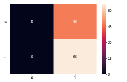
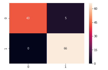
y_predict = svc_model.predict(X_test)
cm = confusion_matrix(y_test, y_predict)

#plotting heatmap
sns.heatmap(cm, annot=True)
print(classification_report(y_test, y_predict))
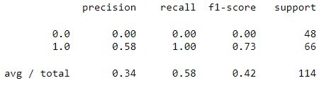
As we can observe from the above results the SVM model fails to detect malignant cases while it detects all the benign cases or we can say that model predicted everything as benign. It means something went wrong during the process.
Let’s try to improve the model by normalizing the data and hyper-parameter tuning of the SVM model.
Model Improvement
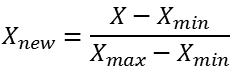
So to improve the model, we have to work on data by performing min-max normalization also known as unity normalization.
min_train = X_train.min()
range_train = (X_train - min_train).max()
X_train_scaled = (X_train - min_train)/range_train

X_train_scaled.head()

As we can see the data is normalized in the range of [0,1]. Next, we have to apply same normalization on test data.
min_test = X_test.min()
range_test = (X_test - min_test).max()
X_test_scaled = (X_test - min_test)/range_test
Now, as we have normalized our training and test set. We can now re build our SVM model on normalized data to see if any improvement happens or not.
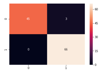
svc_model = SVC()
svc_model.fit(X_train_scaled, y_train)

# model evaluation
y_predict = svc_model.predict(X_test_scaled)
cm = confusion_matrix(y_test, y_predict)

sns.heatmap(cm,annot=True,fmt="d")
print(classification_report(y_test,y_predict))

By observing the above results we can see significant improvement in model performance as it is now able to detect 90% of the malignant cases along with 100% detection of benign cases.
So, from the above experiment, it is clear that the SVM model requires feature scaling to fit well on the data and learn significant features from it.
Next, we will do hyper-parameter tuning of the SVM model to see if it can improve further.
Hyper-parameter Tuning Using Grid Search
Grid search is a technique used in machine learning for hyperparameter optimization. Hyperparameters are manually set variables that are not learned during training.
Grid search works by defining a set of possible values for each hyperparameter and training and evaluating the model for all possible combinations of hyperparameters in a grid-like search space.
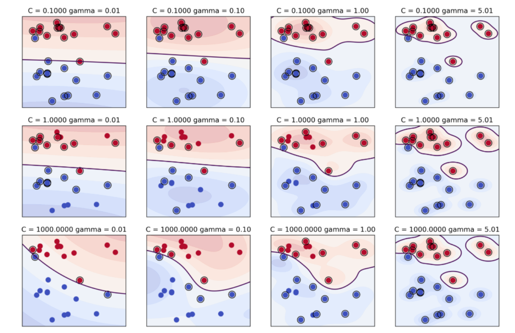
Now let’s start the grid search hyper-parameter tuning by setting kernel as ‘rbf’ which is a non linear kernel.
In support vector machines (SVM), the hyperparameters C and gamma are crucial in determining the performance of the model.
C is the regularization parameter that controls the trade-off between achieving a low training error and a low testing error. A small value of C creates a wider margin hyperplane, allowing for more margin violations but reducing the risk of overfitting. On the other hand, a large value of C creates a narrower margin hyperplane, which reduces margin violations but increases the risk of overfitting.
Gamma, on the other hand, controls the shape of the decision boundary. It defines how far the influence of a single training example reaches, with low values indicating a far reach, and high values indicating a narrow reach. A low gamma value creates a broader curve, leading to a smooth decision boundary, while a high gamma value creates a more complex curve, leading to a decision boundary that is more closely tied to the individual data points.
from sklearn.model_selection import GridSearchCV
param_grid = {'C': [0.1, 1, 10, 100], 'gamma': [1, 0.1, 0.01, 0.001], 'kernel': ['rbf']}
grid = GridSearchCV(SVC(),param_grid,refit=True,verbose=4)
grid.fit(X_train_scaled,y_train)
Now, to check the best hyperparameters obtained from grid search we can simply execute the below code.
grid.best_estimator_

It has given a whole set of optimized hyper-parameters which we can use to build the prediction model.
grid_predictions = grid.predict(X_test_scaled)
cm = confusion_matrix(y_test, grid_predictions)
sns.heatmap(cm, annot=True)
print(classification_report(y_test,grid_predictions))
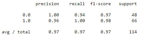
So, now it is evident that after grid search-based hyper-parameter tuning the performance of SVM further improved to 97% from 96% before while recall of malignant cases increased from 90% to 94% which is a significant improvement in this use case.
Ethical Implications of Breast Cancer Prediction
Breast cancer prediction using machine learning has several potential ethical implications. One major concern is the potential for bias in the algorithms used for prediction. If the algorithm is not trained on diverse data that represents all populations, it may not be accurate or fair for all groups. This could lead to unequal access to healthcare and treatment, as well as exacerbate existing health disparities.
Another ethical concern is the privacy and security of patient data. Machine learning algorithms rely on large amounts of data, including personal health information, which could be at risk of being hacked or used for unintended purposes. Additionally, patients may feel uncomfortable with the idea of their data being used for research without their explicit consent.
There is also a risk of over-reliance on machine learning predictions, leading to misdiagnosis or delayed treatment. Physicians and patients must be aware of the limitations of the algorithms and ensure that they are used as a tool to aid in diagnosis and treatment, rather than a replacement for clinical judgement.
Overall, while breast cancer prediction using machine learning has the potential to improve early detection and treatment outcomes, it is important to address these ethical implications to ensure that the benefits are accessible and fair for all patients.
Summary
In summary, we have attempted to predict breast cancer using a numerical dataset by applying a support vector machine (SVM) algorithm. To improve the performance of our model, we first normalized the data, which helped to standardize the range of values and improve the accuracy of the model.
We then performed hyperparameter tuning to find the optimal values of C and gamma. By gradually improving the performance of our model through these techniques, we were able to achieve better accuracy in predicting breast cancer. Overall, our findings suggest that SVM can be a useful tool for predicting breast cancer, and these techniques can help to optimize its performance.