Chronic Kidney Disease Detection using Logistic Regression: A Comprehensive Guide

Chronic kidney disease (CKD) is a critical health issue affecting millions worldwide and can lead to several serious complications. Early detection and treatment can significantly improve patient outcomes. Machine learning has emerged as a powerful tool for predicting CKD in recent years.

In this article, we will demonstrate the use of machine learning algorithm logistic regression for predicting CKD in a step-by-step approach for building an accurate predictive model.

Before deep diving into the implementation of a machine learning model for the prediction of CKD, first, try to understand CKD and its prevalence worldwide.

Understanding Chronic Kidney Disease

Chronic kidney disease is a condition where the kidneys lose their ability to filter waste and excess fluids from the blood leading to a buildup of toxins in the body, which can cause a range of health problems.

CKD is classified into five stages, with stage 1 being the mildest and stage 5 being the most severe. As per the study of the global prevalence of CKD, the current total number of individuals affected by CKD globally was estimated to be 843.6 million.

Chronic kidney disease (CKD) affects approximately 10% of the global population and represents a significant public health challenge. Tragically, millions of individuals succumb to CKD each year, primarily due to a lack of access to affordable treatment options.

CKD has become an increasingly prominent cause of mortality worldwide, as evidenced by its ascent from 27th to 18th place in the Global Burden of Disease study between 1990 and 2010. This rise in prevalence was second only to that of HIV and AIDS.

Although over 2 million people currently receive life-saving dialysis or kidney transplant therapy, this number may only represent a fraction of those who require treatment.

The majority of individuals who do receive treatment reside in just five countries, which account for only 12% of the global population. Conversely, only 20% of patients receive treatment in approximately 100 developing countries which constitute over half of the world’s population.

It is concerning that more than 80% of all individuals receiving treatment for kidney failure reside in wealthy nations with universal healthcare and sizable elderly populations.

Moreover, it is projected that the number of cases of kidney failure will increase disproportionately in developing countries such as China and India, where the elderly population is rapidly expanding.

This trend underscores the urgent need for global strategies to address CKD and promote equitable access to care, particularly in low- and middle-income nations.

Early detection and treatment can help slow down the progression of the disease and prevent complications resulting in a lowering of the mortality rate.

There has been a growing interest in using machine learning (ML) techniques to predict and diagnose chronic kidney disease (CKD). In recent years, several studies have demonstrated the capability of ML algorithms in detecting CKD more accurately compared to traditional methods.

In this article, we will also try to demonstrate the capability of the basic machine learning algorithm Logistic Regression to detect CKD.

Let’s first try to understand the dataset to be used for this project.

Dataset Description

In this project, we have used the Chronic Kidney Disease dataset available on UCI ML Repository. The dataset contains anonymized records of 400 patients with 25 attributes of which 24 are independent features and the remaining one is the target feature determining the CKD status of the patient.

In the CKD dataset, 250 patients have CKD whereas 150 are normal patients. The dataset includes 13 categorical (nominal) features, 11 numeric features, and 1 binary target feature (class).

The attributes of the dataset are described in Table 1 below:

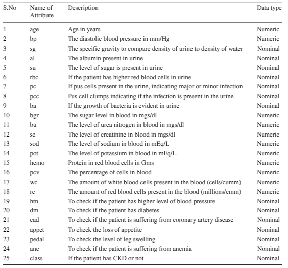
Table 2 below provides an overview of the numerical features in a healthcare dataset, stratified by chronic kidney disease (CKD) status.

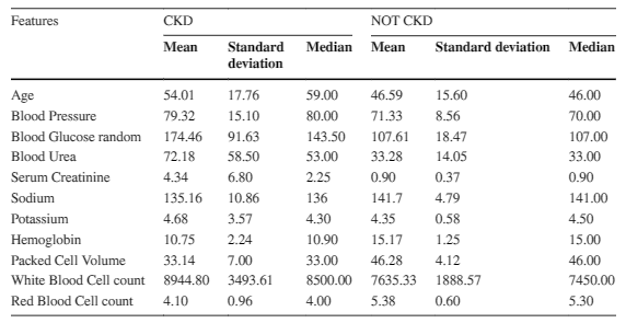
The mean age of CKD patients is 54 years, whereas normal patients have a mean age of 46 years. CKD patients exhibit a significantly higher average blood glucose random level of 174.46 mg/dL compared to the average of 107.61 mg/dL for normal patients.

Additionally, the mean blood urea level for CKD patients is 72.18 mg/dL, which is substantially higher than the mean of 33.26 mg/dL for normal patients. CKD patients also have lower mean hemoglobin levels compared to normal patients.

Moreover, the mean serum creatinine level is notably higher in CKD patients at 4.34 mg/dL versus 0.90 mg/dL for normal patients. Conversely, normal patients have higher mean packed cell volume and red blood cell counts, while CKD patients have lower means for these parameters.

Lastly, the mean white blood cell count in CKD patients is 8944.80 cells/cumm, while normal patients have a relatively lower mean value of 7635.33 cells/cumm.

These findings demonstrate significant differences in clinical characteristics between CKD and normal patients and could aid in the development of predictive models for CKD diagnosis and management.

Importing Python Libraries

The first step is to import all the necessary python libraries required for analysis and building machine learning models.

import pandas as pd
import numpy as np
import matplotlib.pyplot as plt
import seaborn as sns
import plotly.express as px
from sklearn.feature_selection import SelectFromModel
from sklearn.linear_model import LogisticRegression
import warnings
from sklearn import model_selection
from sklearn.model_selection import cross_val_score,train_test_split
from sklearn.feature_selection import SelectKBest
from sklearn.feature_selection import chi2
from sklearn.preprocessing import MinMaxScaler
from sklearn.feature_selection import mutual_info_classif
from sklearn.metrics import classification_report, confusion_matrix
from sklearn.metrics import log_loss,accuracy_score,roc_auc_score,precision_score,recall_score,f1_score
warnings.filterwarnings('ignore')

plt.style.use('fivethirtyeight')
%matplotlib inline
pd.set_option('display.max_columns', 26)

After importing the necessary libraries shown above, we proceed to read the dataset.

Reading Dataset

df= pd.read_csv('kidney_disease.csv')
df.head()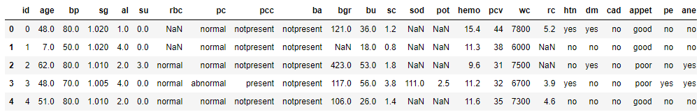

Next, we removed the id column as it is not adding any value to the data and then we further renamed the column names for better readability and understanding of the features.

# dropping id column
df.drop('id', axis = 1, inplace = True)

# rename column names to make it more user-friendly
df.columns = ['age', 'blood_pressure', 'specific_gravity', 'albumin', 'sugar', 'red_blood_cells', 'pus_cell',
              'pus_cell_clumps', 'bacteria', 'blood_glucose_random', 'blood_urea', 'serum_creatinine', 'sodium',
              'potassium', 'haemoglobin', 'packed_cell_volume', 'white_blood_cell_count', 'red_blood_cell_count',
              'hypertension', 'diabetes_mellitus', 'coronary_artery_disease', 'appetite', 'peda_edema',
              'aanemia', 'class']

Checking the Datatype of the features

The next important step is to examine the datatype of all the features so that in case of a discrepancy we can correct them before proceeding to the model-building phase.

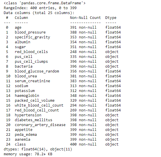
df.info()

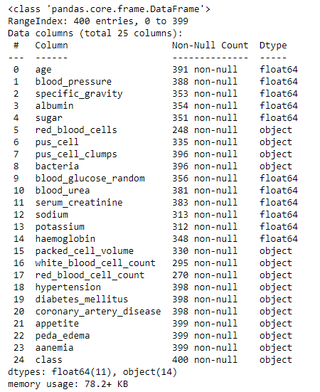
As we can see that 'packed_cell_volume', 'white_blood_cell_count' and 'red_blood_cell_count' are object types. We need to change them to a numerical data type as these are numerical values in general.

# converting necessary columns to numerical type
df['packed_cell_volume'] = pd.to_numeric(df['packed_cell_volume'], errors='coerce')
df['white_blood_cell_count'] = pd.to_numeric(df['white_blood_cell_count'], errors='coerce')
df['red_blood_cell_count'] = pd.to_numeric(df['red_blood_cell_count'], errors='coerce')

df.info()

Data Cleaning

In this step, we tried to clean the data by removing discrepancies and invalid values and characters from the dataset.

For that, we have segregated numerical and categorical values.

# Extracting categorical and numerical columns
cat_cols = [col for col in df.columns if df[col].dtype == 'object']
num_cols = [col for col in df.columns if df[col].dtype != 'object']

# looking at unique values in categorical columns
for col in cat_cols:
    print(f"{col} has {df[col].unique()} values\n")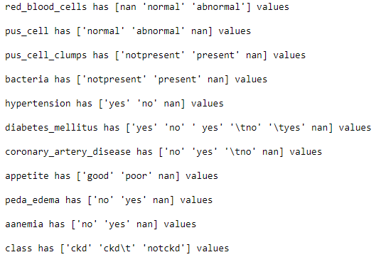

As we can see from the above output, categorical features diabetes_mellitus,coronary_artery_disease, and class have ‘\t’ associated with some of the categories which we have to remove it.

# replace incorrect values

df['diabetes_mellitus'].replace(to_replace = {'\tno':'no','\tyes':'yes',' yes':'yes'},inplace=True)

df['coronary_artery_disease'] = df['coronary_artery_disease'].replace(to_replace = '\tno', value='no')

df['class'] = df['class'].replace(to_replace = {'ckd\t': 'ckd', 'notckd': 'not ckd'})

After handling the ‘\t’, we then need to convert the target variable to numeric values 0,1 instead of notckd and ckd.

df['class'] = df['class'].map({'ckd': 1, 'not ckd': 0})
df['class'] = pd.to_numeric(df['class'], errors='coerce')

Exploratory Data Analysis

Now, in this step, we will do exploratory data analysis by checking the numerical distribution of numeric columns first.

# checking numerical features distribution
plt.figure(figsize = (20, 15))
plotnumber = 1

for column in num_cols:
    if plotnumber <= 14:
        ax = plt.subplot(3, 5, plotnumber)
        sns.distplot(df[column])
        plt.xlabel(column)
        
    plotnumber += 1

plt.tight_layout()
plt.show()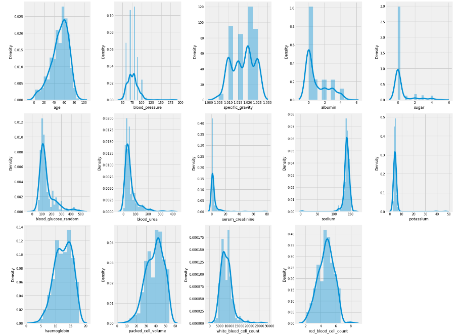

As we can observe from the above histogram of numerical features, it is evident that skewness is present in some of the columns.

Next, we will check the distribution of categorical features.

# looking at categorical columns
plt.figure(figsize = (20, 15))
plotnumber = 1

for column in cat_cols:
    if plotnumber <= 11:
        ax = plt.subplot(3, 4, plotnumber)
        sns.countplot(df[column], palette = 'rocket')
        plt.xlabel(column)
        
    plotnumber += 1

plt.tight_layout()
plt.show()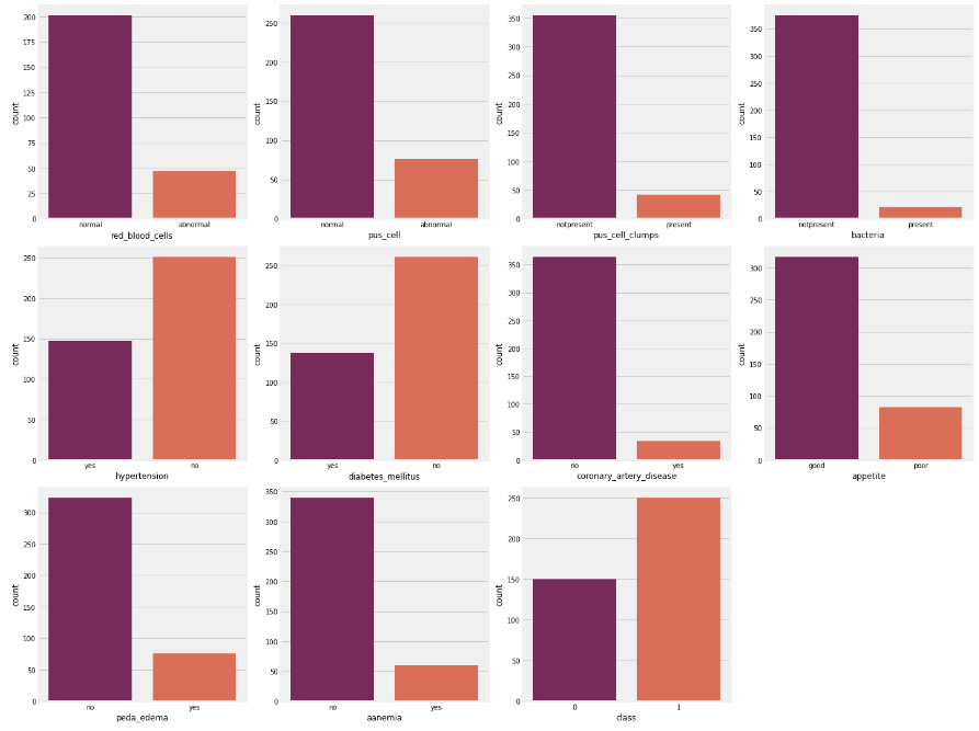

Checking for Multicollinearity

In this step, we will check the multicollinearity among the features by plotting the heatmap.

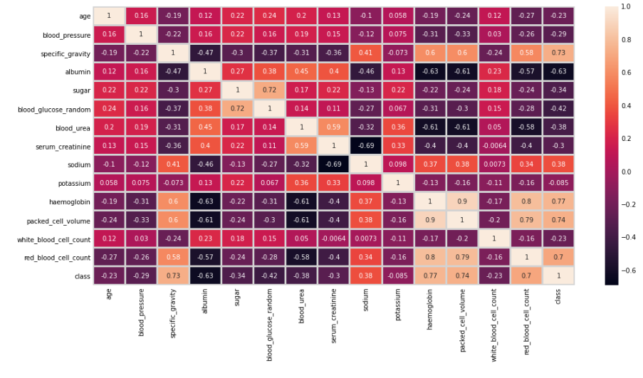
As we can observe from the above plot, the most positively correlated variables are hemoglobin and red_blood_cell_count with a value of 0.8, whereas packed_cell_volume and red_blood_cell_count are the second most correlated variables with a value of 0.79 sugar, whereas serum_creatinine and sodium are highly negatively correlated with a value of -0.69.

We will not remove any highly correlated variables at this stage.

Handling of Missing values

As we know, the Logistic regression algorithm is affected by missing values so we have to handle them in order to build the machine learning model.

For handling missing values we have to first impute missing values in numeric features then will impute missing values in categorical features.

# checking for null values

df.isna().sum().sort_values(ascending = False)

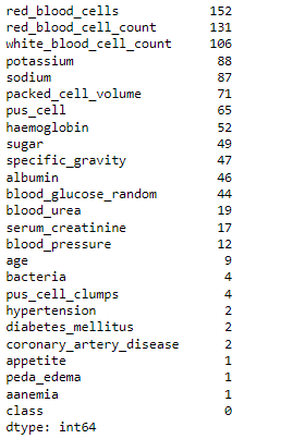
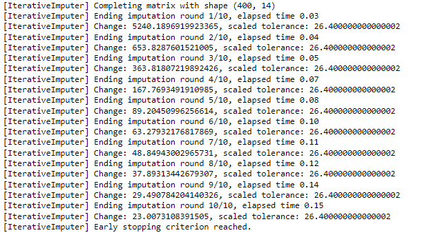
As we can see from the above output, a huge number of missing values are present in the dataset, so we have to handle them using imputation and for that, we will be using the Iterative imputation technique.

#imputation of missing values in numeric features
from sklearn.linear_model import LinearRegression
from sklearn.experimental import enable_iterative_imputer
from sklearn.impute import IterativeImputer

lr = LinearRegression()
imp = IterativeImputer(estimator=lr,missing_values=np.nan, max_iter=10, verbose=2, imputation_order='roman',random_state=0)
df[num_cols]=imp.fit_transform(df[num_cols])

Next, we will segregate features and target variables.

X=df.drop(['class'],axis=1)
y=df['class']

def impute_mode(feature):
    mode = X[feature].mode()[0]
    X[feature] = X[feature].fillna(mode)

def random_value_imputation(feature):
    random_sample = X[feature].dropna().sample(X[feature].isna().sum())
    random_sample.index = X[X[feature].isnull()].index
    X.loc[df[feature].isnull(), feature] = random_sample
    

So for imputing categorical features, we are using two techniques one is mode-based imputation in which the highest frequency value is imputed in the missing values. The second technique is random value imputation.

# filling "red_blood_cells" and "pus_cell" using random sampling method and rest of cat_cols using mode imputation

random_value_imputation('red_blood_cells')
random_value_imputation('pus_cell')

for col in cat_cols[:-1]:
    impute_mode(col)

X[cat_cols[:-1]].isnull().sum()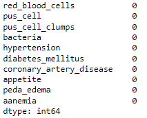

As we can see from the above output there are no missing values left in the dataset. So now we can proceed toward categorical feature encoding.

First, we need to check the number of categories in each categorical variable.

for col in cat_cols:
    print(f"{col} has {df[col].nunique()} categories\n")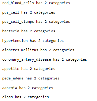

As all of the categorical columns have 2 categories we can use a label encoder.

from sklearn.preprocessing import LabelEncoder

le = LabelEncoder()

for col in cat_cols[:-1]:
    X[col] = le.fit_transform(X[col])

Next, we will proceed to Train Test Split

Train Test Split

# splitting data intp training and test set

from sklearn.model_selection import train_test_split

X_train, X_test, y_train, y_test = train_test_split(X, y, stratify=y,test_size = 0.20, random_state = 0)

Data Normalization

In this step, we will normalize each of the features within a range of 0 to 1 and for that, we will use the Min Max Normalization technique.

minmax = MinMaxScaler()

X_train[num_cols] = minmax.fit_transform(X_train[num_cols])
X_test[num_cols] = minmax.transform(X_test[num_cols])

Model Building and Evaluation

lr =LogisticRegression()
lr.fit(X_train, y_train)

y_pred_lr = lr.predict(X_test)

CM=confusion_matrix(y_test,y_pred_lr)
sns.heatmap(CM, annot=True)

TN = CM[0][0]
FN = CM[1][0]
TP = CM[1][1]
FP = CM[0][1]
specificity = TN/(TN+FP)
loss_log = log_loss(y_test, y_pred_lr)
acc= accuracy_score(y_test, y_pred_lr)
roc=roc_auc_score(y_test, y_pred_lr)
prec = precision_score(y_test, y_pred_lr)
rec = recall_score(y_test, y_pred_lr)
f1 = f1_score(y_test, y_pred_lr)


model_resu =pd.DataFrame([['Logistic Regression',acc, prec,rec,specificity, f1,roc, loss_log]],
               columns = ['Model', 'Accuracy','Precision', 'Sensitivity','Specificity', 'F1 Score','ROC','Log_Loss'])
model_resu

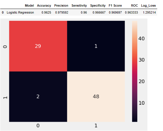
As we can see from the above results, the Logistic regression model is 96.25% accurate in predicting CKD in patients which is a reasonably good model.

Feature Importance

Now to further interpret which features are playing key roles in predicting CKD, we can plot relative feature importance plot for the Logistic Regression model based on the value of its coefficients.

feature_importance = abs(lr.coef_[0])
feature_importance = 100.0 * (feature_importance / feature_importance.max())
sorted_idx = np.argsort(feature_importance)
pos = np.arange(sorted_idx.shape[0]) + .5

featfig = plt.figure()
featax = featfig.add_subplot(1, 1, 1)
featax.barh(pos, feature_importance[sorted_idx], align='center')
featax.set_yticks(pos)
featax.set_yticklabels(np.array(X.columns)[sorted_idx], fontsize=8)
featax.set_xlabel('Relative Feature Importance')

plt.tight_layout()   
plt.show()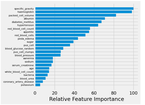

Conclusion

So, in this article, we have shown how to handle such noisy data for building a machine-learning model for detecting chronic kidney disease. Further, we have demonstrated the fitting of the Logistic Regression Model and evaluated its performance. In the end, we have also tried to interpret the model by plotting the relative feature importance plot.

In this, you can explore other machine learning algorithms and compare their performance against benchmark model Logistic Regression.