
Table of Contents
Peer-to-peer lending is the digital marketplace, where borrowers are mapped with investors willing to lend money in the form of investment. P2P lending is evolved from crowd-funding. The basic concept of crowdfunding is that it involves raising capital from a large number of investors to fund a new business venture.
In the recent past, P2P lending emerged as one of the most popular lending options in the US, the UK., Japan, Sweden, Canada, and China.
Due to digital innovation and advancement in information technology, peer-to-peer lending is slowly capturing the finance industry as it is beneficial for both borrowers in the form of cheaper loans and lenders in the form of higher returns.
Peer-to-peer lending provides cheaper loans than any other investment products offered by traditional lending institutions by reducing operating costs and speeding up the lending process with the help of innovative technology.
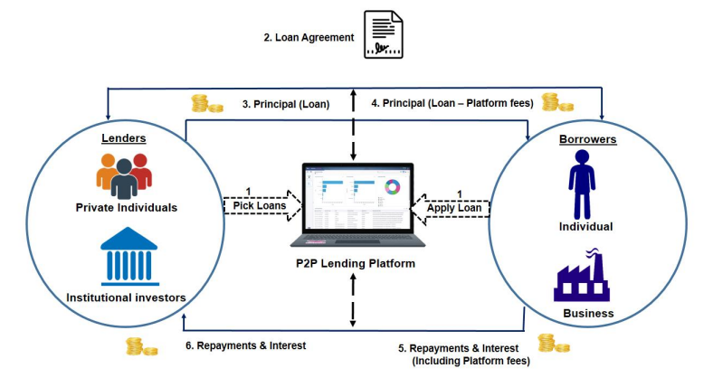
In Fig1. P2P lending is depicted as a six-step process from loan application to loan disbursal.
In the first step, an individual or business entity applies for a loan by registering into the P2P platform, then the platform assigns a credit score to the borrowers based on their credit profile and then loan requirements float into the P2P platform making it available to the investors for investment which acts as a lender.
In the next step, after picking up a loan from an investor, a loan agreement is executed between the lender and the borrower. In this process, the P2P platform acts as a mediator and charges for its services of mapping investors to potential borrowers.
Next, the principal loan amount is deducted from the investor’s account and the platform credits the loan amount to the borrower’s account after deducting its platform fees. In the next step, the borrower starts repaying loans by making payments in the platform which also includes platform fees, and in the end, investors receive funds at the prescribed rate of interest.
Online P2P lending is a convenient solution for borrowers, as it is time-saving and no demand is raised for security by lenders.
But at the same time, it poses a great risk of uncertainty as it is not governed and controlled by regulating authority and transactions are fully online with no face-to-face communication between lenders and borrowers which in turn creates an asymmetry of information.
When a borrower applies for a loan on a P2P lending platform and after sanctioning of the loan, the borrower defaults in repayment of the loan then it may lead to financial loss to the lender and the lender has to suffer due to the default of the borrower.
On the other hand, if the lender does not approve the loan which may be likely to repay by the borrower, then it also leads to financial loss to the lender.
Thus, a system needs to be in place which predicts the stages of defaults of loans by generating Early Warning Signals (EWS) and assessing the creditworthiness of the borrowers to repay the loan in the future through this platform.
Next, we will discuss in detail how we have applied machine learning for predicting the credit risk of the borrowers, and for that, we will first discuss about the dataset we have employed for this project.
Dataset Description
In this work, we have used a publicly available dataset of a leading European peer-to-peer lending platform Bondora owned by the Estonian company Isepankur. They are operational in 23 European countries and their focused target markets are in Spain, Finland, and Estonia.
To date, more than 1.18 lakh investors funded more than 360 million euro loans in the platform, and more than 43 million euro loans were paid out in interest.
The dataset collected from the platform consists of loan applications for a period ranging from March 2009 to January 2020.
The original dataset consists of 112 features with 134529 borrowers. We have selected 33 features that are statistically significant to predict the default of loans.
The distribution of the dataset based on loan status is detailed in Table 1. The dataset can be downloaded from the IEEE data port.
| Status | #Instances |
| Repaid | 31,622 |
| Late | 45,772 |
| Current | 57,135 |
| Total | 1,34,529 |
We further reduce the records of the dataset by selecting only repaid and late status loans as we do have not much more data about the current status of loan(s), which are still operational and not relevant to our research.
So after filtering current status loans and invalid records our final dataset contains 71782 records having 40175 late status loans which we treated as default loans and 31607 as repaid loans that are fully paid by borrowers.
Table 2 provides a description of the features used in the dataset and their data type.
| Feature | Data Type | Description |
| Age | Numeric | Age of borrower in years |
| Gender | Nominal | Gender of the borrower |
| Country | Nominal | Country of borrower |
| Language code | Nominal | Native Language of the borrower |
| Education | Ordinal | Education status of the borrower |
| Marital Status | Nominal | Marital status of the borrower |
| Employment Status | Nominal | Employment status of the borrower |
| Occupation Area | Nominal | Occupation of borrower i.e., in which sector borrower works |
| Home Ownership Type | Nominal | Homeownership status of the borrower |
| Income Total | Numeric | Borrower’s total monthly income |
| Applied Amount | Numeric | The Loan amount applied by the borrower |
| Amount | Numeric | Amount of Loan sanctioned |
| Loan Duration | Numeric | The current duration of the loan in months |
| Interest | Numeric | The maximum interest rate applied in the loan application |
| Monthly Payment | Numeric | The estimated amount the borrower has to pay every month |
| Use of Loan | Nominal | The actual purpose for which the loan was taken by borrower |
| Rating | Ordinal | Bondora Rating issued by the Rating model |
| CreditScoreEsMicroL | Ordinal | A score that is specifically designed for risk classifying subprime borrowers. |
| Debt To Income | Numeric | The ratio of borrower’s monthly gross income that goes toward paying loans |
| Existing Liabilities | Numeric | Borrower’s number of existing liabilities |
| Liabilities Total | Numeric | Total monthly liabilities of borrower |
| Refinance Liabilities | Numeric | The total amount of liabilities of borrower after refinancing |
| No. Of Previous Loans Before Loans | Numeric | Number of previous loans of borrower |
| Amount of Previous Loans Before Loans | Numeric | Value of previous loans of the borrower |
| Previous Repayments before loan | Numeric | How much was the borrower had repaid previous loans prior to this loan |
| Previous early repayment count before loan | Numeric | Number of times borrower repaid the loan early |
| Free Cash | Numeric | Discretionary income of borrower after monthly liabilities |
| Bids Portfolio Manager | Numeric | The amount of investment offers made by Portfolio Managers |
| Bids API | Numeric | The amount of investment offers made via API |
| Bids Manual | Numeric | The amount of investment offers made manually |
| New Credit Customer | Nominal | Did the customer have prior credit history in Bondora. |
| Verification Type | Nominal | The method used for loan application data verification |
| Monthly Payment Day | Numeric | On the day of the month the loan payments are scheduled for |
| Interest and Penalty Payments Made | Numeric | Interest and penalty payments made by borrower so far |
| Employment Duration Current Employer | Ordinal | Employment time of borrower with the current employer |
| Predictor Default | Binary | Default status of the borrower. 0: Loan Repaid, 1: Loan Default |
After necessary pre-processing, we analyzed and calculated correlation coefficients of all the features of the dataset with respect to the default variable using Pearson’s method, and its visual representation is shown in Fig.2.
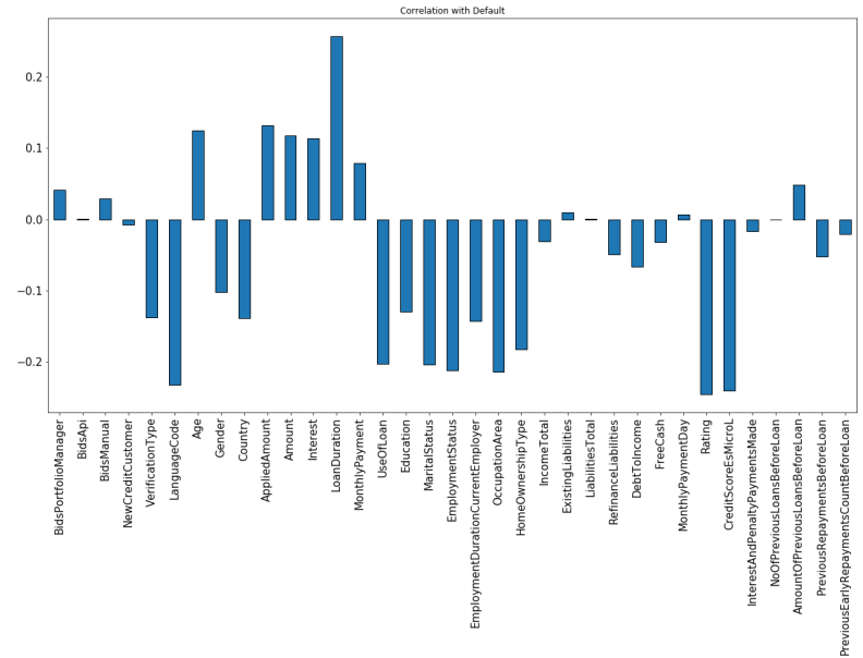
From the figure, we can observe that Loan duration, Applied amount, Sanctioned Amount, and Interest showed a significantly positive correlation with the target variable and among themselves, Loan duration showed the highest positive correlation with the target variable which signifies that shorter duration loans are most likely to be repaid by borrowers in comparison to longer duration loans.
The features, Language Code and Rating are the most negatively correlated variables.
Data Preparation
Data preparation is also known as data pre-processing and it is a very crucial step in building an end-to-end machine learning model. It is the most time-consuming step in the machine learning pipeline as it requires different issues to be addressed in the data before proceeding toward the model-building task.
Data preparation mainly handles two major issues i.e.,
- Impurity in the data (missing records, noise in the data, inconsistent data).
- Generation of quality data as an advanced machine learning algorithm requires quality to generate useful insights. It involves different techniques to generate quality data that can boost the performance of advanced machine learning algorithms such as selecting relevant data also known as feature selection, dimensionality reduction, and constructing new features using domain knowledge, which is also known as feature engineering.
Data Cleaning
Data cleaning is a very important step before building a machine learning-based model. In this research, missing values are handled with a two-step process.
In the first step, a threshold percentage of missing value i.e., 40% in our case selected, and the features which have more than the threshold percentage are simply removed from the dataset.
After removing those features, the dataset was left with 76 features.
In this step further filtering of features by using target relevance methodology i.e., features which have no relevance in default prediction such as Loan ID, Loan Number, Listed on UTC, Username, Bidding Started on, etc., were removed from the dataset.
Apart from that features which add duplicity to the dataset were also removed such as date of birth as the age of the borrower was already present in the dataset and finally, the dataset was left with 47 features.
In the next step, features with less than 40% missing values are handled using the missing value imputation strategy.
In this step, features were segregated into numerical and categorical features. The numerical features having missing values were imputed with median values as they were more representative than mean values for those features whereas in the case of categorical features missing values were imputed with a new category.
Feature Engineering
Feature engineering deals with boosting the performance of machine learning models by transforming the feature space. It is a very important part of data preparation for machine learning.
Its basic purpose is to engineer new features from existing features based on domain knowledge (manual feature engineering) or automatic extraction of new features also known as automatic feature engineering. In this research, we have engineered 5 new features based on credit monitoring. The details of extracted features are shown in Table 3.
| S.No. | Feature | Calculation | Description |
| 1. | Credit length (in months) | Maturity Date Last – Loan Date | This feature determines the total duration of the loan in months as in the case of some borrower’s actual date of repayment was extended due to the current financial condition of the borrower, this extended date is the maturity date last. |
| 2. | Maturity difference (in days) | Maturity date last – Mature date original | This difference gives the intuition about borrower punctuality in repaying the loan on time. It indicates how much borrowers differ from the original repayment terms. |
| 3. | Last Payment days | Maturity date last – Last payment on | This feature is about understanding the gap in the repayment of loan dues. This feature indicates well in advance that borrower chances of default increase as the number of days between the last payment date of the monthly installment and the maturity date of the loan increases |
| 4. | Margin | Applied amount – Loan Amount | It is the difference between the amount applied by the borrower and the actual loan amount issued to the borrower. This difference is also treated as a margin in the conventional banking scenario. |
| 5. | Total asset | Free cash + (Total income – Monthly payment) | It gives the idea of the total asset of the borrower which in turn indicates the borrower’s repayment capability |
Further, detailed summary statistics of the newly engineered feature are shown in Table 4, and later in the result and discussion section, we have compared machine learning models with or without newly created features to understand their importance in predicting default loans.
| Features | Mean | Standard Deviation | Minimum | Maximum |
| credit_length_mnths | 34.5328 | 25.95132 | 0.00 | 130 |
| maturity_diff_days | 48.3200 | 485.9884 | -1855 | 3708 |
| last_paymnt_days | 902.0632 | 703.9819 | -3624 | 2489 |
| diff_amt | 275.8972 | 1121.9921 | -1 | 10450 |
| total_asset | 1944.813 | 6503.415 | -1.070 | 1011781 |
Feature Normalization
Feature normalization is a significant step of data preparation in which features having different scales transform into similar scales.
In this research, the standard scaler method is used for normalizing the data which transforms features such that they have a mean of 0 and a standard deviation of 1.
The standard scaler method is shown in equation 1.
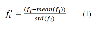
where fi represents an individual feature and fi’ represents a normalized feature.
Feature Transformation
In this work, we have transformed the categorical features using the weight of evidence (WOE) method.
The WOE is a widely used statistical technique for risk assessment and is typically used in the development of credit scorecards. It is an alternative approach to dummy encoding of categorical variables as it substitutes each category of class with a calculated risk value which in turn reduces it down to a single numerical value.
In the context of credit risk analysis, WOE measures the level of separation between the customers who repaid the loan and the ones who default.
The major advantage of WOE is that it handles missing values in categorical features by grouping them into two classes (i.e., repaid and default) and assigning the numerical value based on their distribution in both classes which is a relatively more effective method than the conventional strategy of creating a new category for handling missing values.
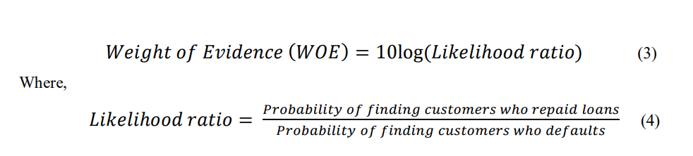
The numerical definition of WOE in terms of credit risk assessment is defined below in equation 2:
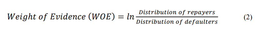
WOE transformation is a commonly used transformation technique that works well with the logistic regression-based credit risk model as both use the concept of log odd ratio.
WOE is also defined numerically in terms of likelihood ratio as follows (Smith et.al, 2002):
Exploratory Data Analysis
Exploratory data analysis is a very important step for getting a qualitative understanding of the dataset. It involves statistical analysis of data along with data visualization which helps in visualizing relationships within features, distribution of features, and understanding patterns and trends in the data using graphical plots.
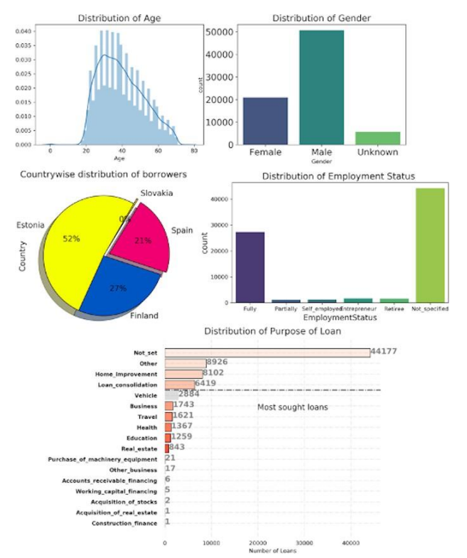
In Fig. 4 we have summarized the distribution of different features. In the first four figures, demographic features are summarized while the last figure depicted the main purpose of loans.
As we can see from the figure most of the loans were given in the age group of 25 – 45 years whereas the majority of borrowers were male. Apart from that, more than 50% of borrowers belong to the country Estonia and a maximum number of loans comprise borrowers who have not specified their employment status.
It is evident from the figure that most of the loans given to borrowers for unspecified purposes may be in the form of personal loans while another most sought purpose of loans was other, home improvement and loan consolidation.
Methodology
1. Logistic regression as meta-learner
In this project, logistic regression was used as the meta-learning algorithm for the prediction of default rates.
As credit risk prediction is a multivariate classification problem with binary independent variables where 0 represents fully paid loans and 1 represents default loans, multinomial logistic regression is used to estimate the probability of default loans.
2. Two-level stack ensemble framework
The stacked ensemble is also known as Super Learning. This technique is used to ensemble a diverse set of machine learning algorithms to improve the overall performance of the resultant model.
This technique proved successful in many popular machine learning competitions, such as the Netflix competition, KDD cup, and Kaggle competitions.
Unlike bagging and boosting, stacking is generally a heterogeneous combination of learners. The basic idea here is to use the level-1 model to learn from the predictions of base models at level-0. The working principle of stacking is depicted in the below algorithm as a stepwise process as follows:
Step 1. Selecting the list of base algorithms say M.
Step 2. Selecting meta-learning algorithm
Step 3. Splitting the training set into k-folds for performing cross-validation on the training set
Step 4. All the base algorithms are fitted on the k-1 part of the training data whereas the kth part is used for prediction.
Step 5. The N cross-validated values of base algorithms are captured and a matrix of order M x N is formed.
This M x N matrix is treated as Level one data which acts as training data for the meta-learning algorithm.
Step 6. Meta-learning algorithm to be trained on the above Level one data which can be further used to generate predictions on the test set.
In this framework, Random Forest, Extra Tree Classifier, Adaboost, Gradient boosting machine (GBM), extreme gradient boosting (XGBoost), and Light Gradient Boosting Machine (LGBM) were used as level 1 models while logistic regression was used as level 2 model.
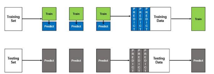
3. Two-level blending framework
Blending is relatively similar to stacked generalization, the only difference is that in stacking cross-fold validation is used to train the individual base learners whereas in blending a small hold-out set or validation set is used to train individual learners.
The final meta-classifier then trains on this validation set only. The general architecture of blending is shown in Fig.5.
In this method, we have used the same base-level algorithms which have been used in the stacking framework while the meta-classifier is also logistic regression in this case.
4. Soft Voting Ensemble Framework
In the soft voting method, each classifier should be well-calibrated i.e., the classifier should output prediction in the form of probabilities for each class which is defined in the following equation:
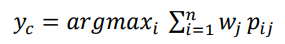
In the above equation, wj is the weight assigned to jth classifier whereas pij is the prediction<br>probability of jth classifier for ith class.
In this study, we divided the dataset into train and test sets in the ratio of 80:20 i.e., 80% of the data was used to train the models, and the rest 20% of the data was utilized to evaluate them using different evaluation metrics such as Confusion matrix, Precision, Recall, F1-Measure, AUC, True Positive Rate, True Negative Rate, Kolmogorov Smirnov statistics, and Gini Index.
Kolmogorov Smirnov or K-S statistics measure the maximum separation in terms of<br>percentage between good borrowers and bad borrowers captured by the model in cumulative distributions of good and bad borrowers. Its value ranges between 0 and 1 and is given by the equation:
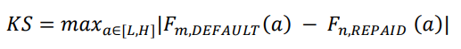
where n is the number of repaid loans and m is the number of default loans. L is the minimum value of the score and H is the maximum value. Fm (a), Fn (a) are the cumulative distribution function of scores for default and repaid loans respectively.
In economics, Gini Index was created to measure income inequality. In the context of credit risk modeling, Gini is utilized with the same purpose to measure inequality between non-defaulted or good borrowers and defaulted or bad borrowers in a population.
The Gini Index is measured by plotting the cumulative proportion of defaulted or bad borrowers as a function of the cumulative proportion of all borrowers.
Its value ranges between 1 and -1 where 1 is the ideal score which perfectly separates the good borrower and bad borrower and 0 is the random score assigned to the borrower.
Result and Analysis
In this section, we have presented the detailed result of our experiment. In this study, after building different ensemble machine learning models, 5-fold stratified cross-validation was performed to estimate the performance of machine learning models to be used as base learners for stacking, blending, and soft voting method.
In 5-fold cross-validation, the entire training data was randomly partitioned into 5 equal subsamples in which one sample was used for validation and the remaining 4 samples were used to train the model.
The process was repeated 5 times i.e., the number of folds, with every 5 subsamples used once for validating the model.
The results from 5 folds averaged to estimate the performance of the model.
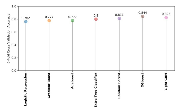
Figure 6. shows the averaged 5-fold cross-validation accuracy of machine learning models used as a base<br>learner in which XGBoost achieved the highest accuracy of 84.4% while LightGBM achieved the second-highest accuracy of 82.5%.
As Logistic regression is a simple model that achieved the lowest accuracy of 76.2% whereas Gradient boost and Adaboost perform slightly better with an accuracy of 77.7%.
In Table 6. the confusion matrix of stacking, blending, and soft voting is shown. As per the table, stacking performed significantly better in terms of predicting non-defaulters while soft voting performed better in terms of classifying default loans.
However, the blending model showed significantly better results in classifying non-defaulters than the soft voting model.
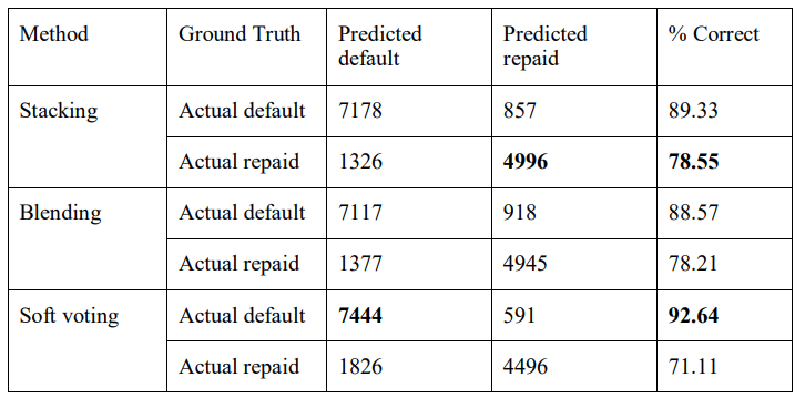
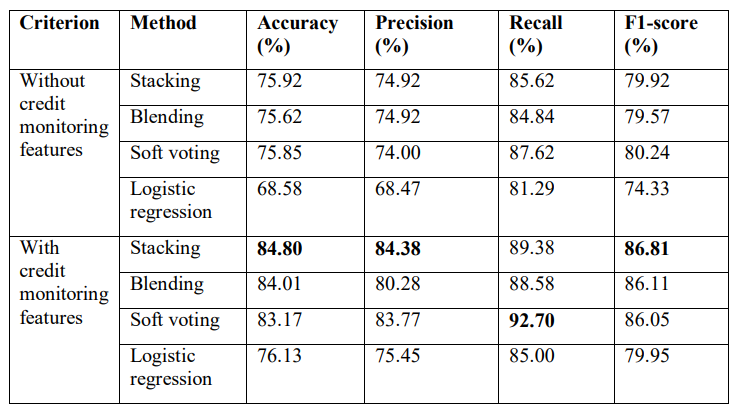
Table 7 summarizes the performance of stacking, blending, and soft voting with or without<br>credit monitoring features on the test set in terms of different evaluation metrics i.e., Test<br>Accuracy, Precision, Recall, and F1-score.
The result shows that with handcrafted credit monitoring features the accuracy of all ensemble models increased to more than 9% and in the case of even simple logistic regression accuracy increased to 8% while the precision, recall, and f1- score of ensemble models increased to more than 5% whereas significant improvement in performance observed in case of a simple logistic regression model.
In the absence of credit, monitoring features stacking attained the highest accuracy and precision while soft voting performed well in terms of recall and f1-score.
With credit monitoring features in place, stacking showed the best performance in terms of accuracy, precision, and f1-score while soft voting performed relatively well in detecting default borrowers as it achieved the highest recall of 92.70%.
For selecting the most robust model, we have<br>employed broadly used evaluation metrics in the credit risk modeling domain i.e.,<br>Kolmogorov Smirnov or KS Statistics, Gini index for testing the discriminatory power of<br>the models, and Average Area Under the Curve (AUC) for comparing the generalization<br>the capability of the model.
Figure 7 demonstrated the Reciever Operating Characteristics
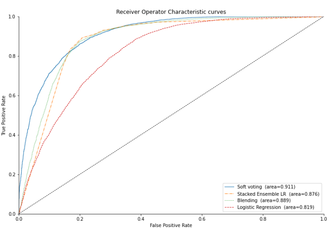
ROC Curves corresponding to the three ensemble models i.e., stacking, blending, and soft voting, and simple logistic regression model, show true positive rate vs false positive rate at various threshold levels.
The closer the curve follows the path in the direction of top-left the region, the more generalized the modeling method is.
The ROC curve of the soft voting model followed the extreme top-left path and achieved the highest AUC value of 91.1% which outperformed other modeling approaches.
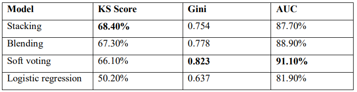
From Table 8 we can observe that the soft voting model achieved the highest Gini index of 0.823 along with the highest AUC while in terms of K-S statistics, it scored a satisfactory score of 66.1% better than the simple logistic regression model while slightly less than stacking which scored 68.4%.
As per the above results, the soft voting model performed relatively well in all the performance measures and achieved the highest performance in terms of Recall, AUC, and Gini Index which led to the conclusion that the soft voting model has the highest predictive power and relatively more generalized in classifying default loans in peer-to-peer lending.
As per the results, the simple logistic regression model performed not up to a satisfactory level in all the evaluation metrics with or without credit monitoring features.
Based on the soft voting model we have plotted a weighted average feature importance plot highlighting the top 20 contributing features as shown in Figure 8.
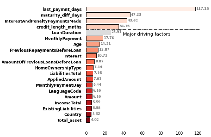
The Feature importance plot showed that features last_paymnt_days, maturity_diff_days, InterestsAndPenaltyPaymentsMade, credit_length_mnths, and loan_duration have the highest importance in predicting default loans which suggest that these features strongly influence the output of the soft voting model.
Hence, from the results, it can be concluded that credit monitoring features are relatively more contributing than demographic features in the prediction of credit risk.
Conclusion
The demonstrated soft voting-based credit risk model with engineered credit monitoring features showed significant results in the prediction of credit risk in the peer-to-peer lending market.
The study also showed that ensemble methods outperform traditional credit risk models based on logistic regression.
The credit risk model shown in this study can assist P2P lenders in predicting default loans in advance once the loan is sanctioned and disbursed to the borrower.
This model can be helpful to lenders in taking wise decisions by analyzing the repayment habits of the borrower which in turn assists them in taking preventive measures to reduce the possibility of credit risk by offering suitable relaxation to the borrower.
This study showed the applicability of the ensemble-based credit risk model in the P2P lending market which can be<br>further extend to the commercial banking market.