
Table of Contents
Medical insurance is a crucial aspect of healthcare and financial planning. In the past, individuals relied on the offline way i.e., insurance agents to predict the amount they should pay in premiums for medical insurance. Health insurance premiums are dependent on various factors like existing diseases, historical diseases, age, BMI, physical fitness, etc. In this article, we have demonstrated step-by-step medical insurance premium prediction using machine learning in Python using the open-source dataset available on Kaggle.
Predicting medical insurance premium is important for both individuals as well as insurance companies. According to data from the U.S. Census Bureau, approximately 91% of the U.S. population had health insurance coverage in 2019.
The above stats signifies that a large portion of the US population relies on health insurance to cover their medical expenses. Therefore, accurate prediction of health insurance premiums is important for individuals as it helps them to carefully plan for medical expenses in advance and ensure that they are adequately covered for any medical emergencies. Furthermore, it can also help individuals to choose the right insurance policy and ensure that they are getting value for their money.

For insurance companies, accurate prediction of health insurance premiums is significant for maintaining profitability and minimizing financial losses. It can also help insurance companies to identify individuals who are at higher risk of filing claims, leading to better risk assessment and management.
Comparison with Traditional Methods
In comparison to traditional methods, such as actuarial tables or underwriting guidelines, machine learning has the potential to be more accurate and efficient.
Actuarial tables and underwriting guidelines are often based on generalizations and assumptions, whereas machine learning algorithms can account for individual differences and nuances in the data.
Additionally, machine learning can continuously adapt and improve over time as it is fed more data, whereas traditional methods may become outdated or less accurate over time.
However, it is important to note that machine learning is not a panacea and can still be subject to biases and errors. It is important to carefully evaluate and validate the algorithms and the data used to train them to ensure that they are fair, accurate, and unbiased.
Understanding Dataset
In this project, we will be using an Insurance Premium Prediction dataset that is available on Kaggle. The dataset consists of 7 columns, which are age, sex, BMI, children, smoker, region, and expenses. The expenses column is the predictor variable that we need to predict using machine learning algorithms.
The age column contains the age of the insured individual, while the sex column indicates whether the individual is male or female. The BMI column contains the Body Mass Index of the insured individual, which is a measure of body fat based on height and weight. The children column indicates the number of children that the individual has, while the smoker column indicates whether the individual is a smoker or not. The region column indicates the region in which the individual lives.
Let’s look at the snapshot of the dataset to better understand it.
import numpy as np # linear algebra
import pandas as pd # data processing, CSV file I/O (e.g. pd.read_csv)
import seaborn as sns
import pandas as pd
import matplotlib.pyplot as plt
%matplotlib inline
import os

df=pd.read_csv('insurance.csv')
df.head()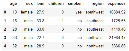
As we can see from the above snapshot the dataset has three numerical columns and three categorical columns except for expenses which is our predictor variable.
Exploratory Data Analysis (EDA)
Next, we will do a basic exploration of the dataset to understand the underlying pattern within the dataset.
df.info()
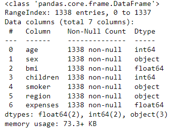
As we can see from the above stats, the dataset has 1338 records and there are no null values in the dataset which is good news for us.
Distribution of Target Variable
In this, we will see the distribution of the target variable to understand if there is any outlier present in the dataset or not.
# Get the label column
label = df[df.columns[6]]

# Create a figure for 2 subplots (2 rows, 1 column)
fig, ax = plt.subplots(2, 1, figsize = (9,12))

# Plot the histogram
ax[0].hist(label, bins=100)
ax[0].set_ylabel('Frequency')

# Add lines for the mean, median, and mode
ax[0].axvline(label.mean(), color='magenta', linestyle='dashed', linewidth=2)
ax[0].axvline(label.median(), color='cyan', linestyle='dashed', linewidth=2)

# Plot the boxplot
ax[1].boxplot(label, vert=False)
ax[1].set_xlabel('Price')

# Add a title to the Figure
fig.suptitle('Premium Distribution')

# Show the figure
fig.show()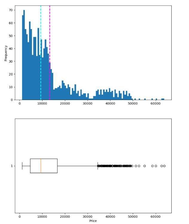
As we can see from the above plot, the expenses column has a few outliers present that we need to remove in order to build a robust machine-learning regression algorithm. The records having a premium amount > 50000 are clearly outliers.
df = df[df['expenses']<50000]
# Get the label column
label = df[df.columns[6]]

# Create a figure for 2 subplots (2 rows, 1 column)
fig, ax = plt.subplots(2, 1, figsize = (9,12))

# Plot the histogram
ax[0].hist(label, bins=100)
ax[0].set_ylabel('Frequency')

# Add lines for the mean, median, and mode
ax[0].axvline(label.mean(), color='magenta', linestyle='dashed', linewidth=2)
ax[0].axvline(label.median(), color='cyan', linestyle='dashed', linewidth=2)

# Plot the boxplot
ax[1].boxplot(label, vert=False)
ax[1].set_xlabel('Label')

# Add a title to the Figure
fig.suptitle('Premium Distribution')

# Show the figure
fig.show()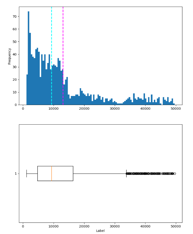
Now the expenses column is well distributed.
Correlation Plots
Next, we will examine the correlation between numerical features and the expenses column.
num_cols=['age','bmi','children']
for col in num_cols:
    fig = plt.figure(figsize=(9, 6))
    ax = fig.gca()
    feature = df[col]
    correlation = feature.corr(label)
    plt.scatter(x=feature, y=label)
    plt.xlabel(col)
    plt.ylabel('Correlations')
    ax.set_title('Expenses vs ' + col + '- correlation: ' + str(correlation))
plt.show()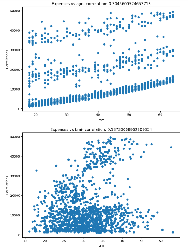
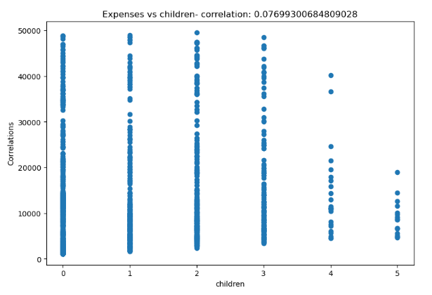
As we can see from the above correlation plots, the expenses column is most correlated with the age column which is pretty obvious.
Feature Encoding
In this step, we will encode categorical features into numerical values as machine learning algorithms can only understand numerical data.
So, first, we will encode features having binary or 2 values i.e, sex and smoker.
sex = {'male': 1,'female': 0}
smoker = {'yes': 1,'no': 0}

df.sex = [sex[item] for item in df.sex]
df.smoker = [smoker[item] for item in df.smoker]
For the region, we have to do one hot encoding as it contains more than 2 categories.
##  one hot encoding region
dummies_r = pd.get_dummies(df["region"], prefix="region")
df = pd.concat([df,dummies_r], axis=1)
df = df.drop("region", axis=1)
Feature and Target Segregation
Next, we will segregate the feature and target variable for training the machine learning algorithm
X = df.drop(['expenses'],axis=1)
y=df['expenses']
Train Test Split
Now, we will do Training and Test split by 80:20 ratio.
from sklearn.model_selection import train_test_split
# Split data 70%-30% into training set and test set
X_train, X_test, y_train, y_test = train_test_split(X, y, test_size=0.20, random_state=0)
Feature Normalization
In this step, we will normalize the numerical features in the range of [0,1] using the min-max scaler function in sklearn.
from sklearn.preprocessing import MinMaxScaler
minmax = MinMaxScaler()

X_train[num_cols] = minmax.fit_transform(X_train[num_cols])
X_test[num_cols] = minmax.transform(X_test[num_cols])
Model Building
Now, as we have done all the basic data pre-processing required for building a regression model, let’s start by building Linear regression as our base model.
1. Linear Regression Model
from sklearn.linear_model import LinearRegression
from sklearn.metrics import mean_squared_error, r2_score
import numpy as np

# Fit a linear regression model on the training set
model = LinearRegression().fit(X_train, y_train)

predictions = model.predict(X_test)
np.set_printoptions(suppress=True)
print('Predicted labels: ', np.round(predictions)[:10])
print('Actual labels   : ' ,y_test[:10])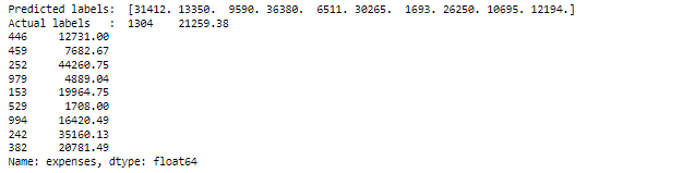
Visualizing Regression Line
plt.scatter(y_test, predictions)
plt.xlabel('Actual Labels')
plt.ylabel('Predicted Labels')
plt.title('Daily Bike Share Predictions')
# overlay the regression line
z = np.polyfit(y_test, predictions, 1)
p = np.poly1d(z)
plt.plot(y_test,p(y_test), color='magenta')
plt.show()


mse = mean_squared_error(y_test, predictions)
print("MSE:", mse)

rmse = np.sqrt(mse)
print("RMSE:", rmse)

r2 = r2_score(y_test, predictions)
print("R2:", r2)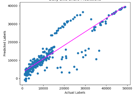
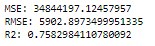
As we can see the linear regression model is pretty average having an R2 score of 0.75. Next, we will try some advanced regression models to see if we can improve the performance of the model.
2. Random Forest Regressor
from sklearn.ensemble import RandomForestRegressor

# Train the model
model_rf = RandomForestRegressor().fit(X_train, y_train)
print (model_rf, "\n")

# Evaluate the model using the test data
predictions = model_rf.predict(X_test)
mse = mean_squared_error(y_test, predictions)
print("MSE:", mse)
rmse = np.sqrt(mse)
print("RMSE:", rmse)
r2 = r2_score(y_test, predictions)
print("R2:", r2)

# Plot predicted vs actual
plt.scatter(y_test, predictions)
plt.xlabel('Actual Labels')
plt.ylabel('Predicted Labels')
plt.title('Daily Bike Share Predictions')
# overlay the regression line
z = np.polyfit(y_test, predictions, 1)
p = np.poly1d(z)
plt.plot(y_test,p(y_test), color='magenta')
plt.show()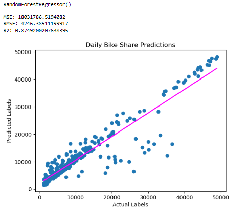
As we can see random forest regressor has shown significant performance by attaining an R2 score of 0.87 whereas RMSE of 4246.38 and MSE of 18021786 are also lesser than linear regression RMSE and MSE respectively.
Feature Importance
From the above results, we have found that the Random Forest regressor showed significant results in predicting health insurance premiums so we will now plot feature importance plot as random forest supports feature importance.
def plot_feature_importance(importance,names,model_type):
    feature_importance = np.array(importance)
    feature_names = np.array(names)

#Create a DataFrame using a Dictionary
    data={'feature_names':feature_names,'feature_importance':feature_importance}
    fi_df = pd.DataFrame(data)

#Sort the DataFrame in order decreasing feature importance
    fi_df.sort_values(by=['feature_importance'], ascending=False,inplace=True)

#Define size of bar plot
    plt.figure(figsize=(10,8))
#Plot Searborn bar chart
    sns.barplot(x=fi_df['feature_importance'], y=fi_df['feature_names'])
#Add chart labels
    plt.title(model_type + 'FEATURE IMPORTANCE')
    plt.xlabel('FEATURE IMPORTANCE')
    plt.ylabel('FEATURE NAMES')

rf = RandomForestRegressor()
rf_fit = rf.fit(X_train, y_train)

feature_importances = rf_fit.feature_importances_

plot_feature_importance(rf_fit.feature_importances_,X_train.columns,'RANDOM FOREST')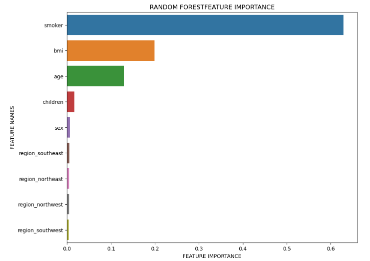
Based on the above plot, it is evident that in the Random Forest model, the top 3 features which influence the health insurance premium the most are Smoker, BMI, and Age.
Ethical Implications of Using Machine Learning for Medical Insurance Premium Prediction
There are several potential ethical implications of using machine learning to predict health insurance premiums. One major concern is that the use of such algorithms could result in unfair or discriminatory practices. For example, if the algorithm is trained on historical data that contains biases or reflects existing disparities, it could perpetuate those biases and result in certain groups being unfairly denied coverage or charged higher premiums.
Another concern is the potential for invasion of privacy, as the use of personal data such as medical history and lifestyle habits to predict insurance premiums could be seen as intrusive or unethical. There is also the risk that the algorithms could be used to target individuals with specific health conditions, which could have negative consequences for their health and well-being.
Finally, there is the risk that the use of machine learning to predict health insurance premiums could exacerbate existing inequalities in access to healthcare. If insurance companies use the algorithms to target only certain groups or areas, it could lead to a concentration of resources in those areas, leaving other regions underserved.
Overall, it is important to carefully consider the potential ethical implications of using machine learning to predict health insurance premiums and to take steps to ensure that these algorithms are fair, transparent, and respectful of individuals’ privacy and rights.
Conclusion
In conclusion, this project has explored the health insurance dataset to predict insurance premiums using machine learning algorithms. Through the exploration process, we gained a better understanding of the dataset and performed basic exploratory data analysis and data preprocessing.
We then trained linear regression and random forest regressor models to predict the insurance premiums. During the model comparison, we found that the random forest regressor model performed better than the linear regression model. By plotting the feature importance plot, we found that smoker, BMI, and age are the top three features that influence the premium value in general.
This project demonstrates the effectiveness of machine learning algorithms in predicting health insurance premiums and highlights the importance of accurate premium prediction for both individuals and insurance companies. In last, we also discussed what will be the potential ethical implications of using machine learning for health insurance premium prediction.