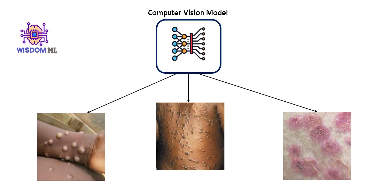
In this article, we will demonstrate a deep learning approach for the detection of Monkeypox disease from skin lesion images. But before proceeding with the model-building process we should know what is Monkeypox disease. how it can spread? and how much serious it is in terms of fatality rate?

About Monkeypox disease

Monkeypox is a skin-related disease that is caused by a zoonotic virus i.e, it transmits from animals to animals and animals to humans. Monkeypox primarily affects rodents, rats, mice, or monkeys. But it can also occur in humans due to close contact with the infected animals or already infected person or with material contaminated with the virus.

The symptoms of Monkeypox are somewhat similar to smallpox and its primarily prevalent in Central and West Africa but due to international travel, import-export of animals, and physical contact with an infected animal or person it is also spreading in other regions such as the U.K., U.S., Australia, Portugal, Spain, Canada, etc.

Monkeypox is a self-limiting disease and it usually lasts 2 to 4 weeks. But recently it is spreading at an alarming rate with a fatality ratio of 3 to 6%. Early detection of Monkeypox can help doctors in limiting the disease and increasing the chances of saving human lives.

In this article, we will demonstrate the training of computer vision-based transfer learning model MobileNetV2 on an open source dataset available on Kaggle and compare their performance.

Dataset used

In this project, we have used Monkeypox Skin Lesion Dataset available on Kaggle. In this dataset along with the ‘Monkeypox’ class, skin lesion images of ‘Chickenpox’ and ‘Measles’ are also included. So it’s a binary classification dataset in which one class belongs to Monkeypox whereas another class labeled as ‘Others’ consists of Chickenpox and Measles images. Further, the dataset has the following 3 folders:

1) Original Images: It contains a total number of 228 images of which 102 belong to the ‘Monkeypox’ class and the remaining 126 belong to the ‘Others’ class i.e., (chickenpox and measles) cases.

2) Augmented Images: This folder consists of augmented images in both classes. In this images are augmented using different augmentation techniques: rotation, translation, reflection, shear, hue, saturation, contrast and brightness jitter, noise, scaling, etc.

3) Fold1: This folder is one of the three-fold cross-validation datasets. The original images were split into training, validation, and test set(s) with the approximate proportion of 70: 10: 20. In this only the training and validation images are augmented while the test set consists of original images.

In this project, we have used the Fold1 dataset for training our computer vision models.

The distribution of images in Train, Val, and Test under the Fold 1 folder is given below:

1. Train: Monkeypox – 980 and Others -1,162
2. Val: Monkeypox – 168 and Others -252
3. Test: Monkeypox – 20 and Others -25

Importing libraries

In this step, we will import important libraries required during the model training and evaluation process.

import pandas as pd
import numpy as np
import cv2                     
import os                  
from random import shuffle
import random
#for preprocessing
from tensorflow.keras.preprocessing import image
import matplotlib.pyplot as plt
from tensorflow.keras.utils import to_categorical
from tensorflow.keras.models import Sequential
from tensorflow.keras.layers import Conv2D,MaxPooling2D,Dense,Flatten,Dropout  
from tensorflow.keras.callbacks import EarlyStopping, ModelCheckpoint, ReduceLROnPlateau
from random import shuffle
#For augmentation
from tensorflow.keras.preprocessing.image import ImageDataGenerator
#Transfer learning models
from tensorflow.keras.applications.mobilenet_v2 import MobileNetV2
from tensorflow.keras import Model, layers
from numpy import loadtxt
import itertools
from sklearn.metrics import confusion_matrix,classification_report
from tensorflow.keras.applications.imagenet_utils import preprocess_input, decode_predictions
from tensorflow.keras.models import load_model

In the next step, we will set the directory and check some sample images in the dataset

# setting path of directory
M_DIR =  "/content/drive/MyDrive/Monkey_Pox_Dataset/Train/Monkeypox/"
O_DIR = "/content/drive/MyDrive/Monkey_Pox_Dataset/Train/Others/"


# storing all the files from directories M_DIR and O_DIR to Mimages and Oimages for accessing images directly

Mimages = os.listdir(M_DIR)
Oimages = os.listdir(O_DIR)

sample_monkeypox = random.sample(Mimages,6)
f,ax = plt.subplots(2,3,figsize=(15,9))

for i in range(0,6):
    im = cv2.imread(M_DIR +sample_monkeypox[i])
    ax[i//3,i%3].imshow(im)
    ax[i//3,i%3].axis('off')
f.suptitle('Monkeypox sample images',fontsize=20)
plt.show()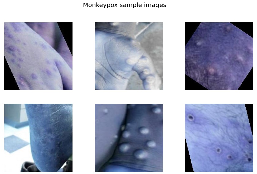

sample_others = random.sample(Oimages,6)
f,ax = plt.subplots(2,3,figsize=(15,9))

for i in range(0,6):
    im = cv2.imread(O_DIR +sample_others[i])
    ax[i//3,i%3].imshow(im)
    ax[i//3,i%3].axis('off')
f.suptitle('Others sample images',fontsize=20)
plt.show()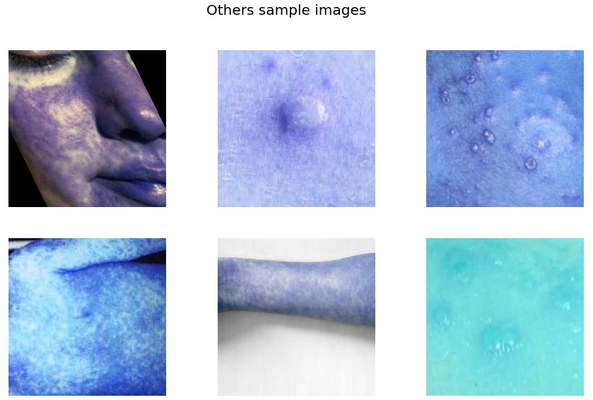

From the sample images, we get the initial level intuition that rashes in the case of Monkeypox are quite serious and mostly spread on hands, feet, and mouth whereas other diseases have even spread rashes to the whole body.

Data Preparation – Loading Images and Labels

In this step, we will load the image data for training the computer vision-based CNN model.

data=[]
labels=[]
for m in Mimages:
    try:
        image=cv2.imread(M_DIR+m)
        image_from_array = Image.fromarray(image, 'RGB')
        size_image = image_from_array.resize((224, 224))
        data.append(np.array(size_image))
        labels.append(1)
    except AttributeError:
        print("")

for o in Oimages:
    try:
        image=cv2.imread(O_DIR+o)
        image_from_array = Image.fromarray(image, 'RGB')
        size_image = image_from_array.resize((224, 224))
        data.append(np.array(size_image))
        labels.append(0)
    except AttributeError:
        print("")

#converting features and labels in array
feats=np.array(data)
labels=np.array(labels)

# saving features and labels for later re-use
np.save("/content/drive/My Drive/skin_cancer_dataset/feats_train",feats)
np.save("/content/drive/My Drive/skin_cancer_dataset/labels_train",labels)

As you can see from the code, we are first reading the images of both the class, resizing them to a size of (224,224), and later converting them into a NumPy array so that we can save them for later re-use. By saving images into the NumPy array we can reduce the loading time in comparison to image data.

As we have saved the image data as NumPy arrays now we can load it for further processing.

feats=np.load("/content/drive/MyDrive/Monkey_Pox_Dataset/feats_train.npy")
labels=np.load("/content/drive/MyDrive/Monkey_Pox_Dataset/labels_train.npy")

s=np.arange(feats.shape[0])
np.random.shuffle(s)
feats=feats[s]
labels=labels[s]

num_classes=len(np.unique(labels))
len_data=len(feats)

As we can see from the above code, after loading the data we are also shuffling it so that it cannot be sequentially arranged before training the model. the data should be randomly distributed among classes so that model will be trained without bias.

Train Test Split

In this step, we will divide the dataset into training and test sets in the ratio of 80:20.

# splitting dataset into 80:20 ratio i.e., 80% for training and 20% for testing purpose
(x_train,x_test)=feats[(int)(0.2*len_data):],feats[:(int)(0.2*len_data)]

(y_train,y_test)=labels[(int)(0.2*len_data):],labels[:(int)(0.2*len_data)]

Image Normalization

In this step, we will normalize the images by dividing them by 255.

x_train = x_train.astype('float32')/255 # As we are working on image data we are normalizing data by divinding 255.
x_test = x_test.astype('float32')/255
train_len=len(x_train)
test_len=len(x_test)


#Doing One hot encoding as classifier has multiple classes
y_train=to_categorical(y_train,num_classes)
y_test=to_categorical(y_test,num_classes)

Model Building

As we have a small dataset so in this project we will be employing a transfer learning approach by finetuning a pre-trained MobileNetV2. So, first, we have to download the imagenet weights of the Mobilenet model.

So, as we can observe in the below code we are only making the base layers trainable while the top layers as trainable False i.e., we will be utilizing the basic image classification capability of the Mobilenet V2 model which is trained on imagenet dataset.

Next, we will add additional layers for customizing the model for our task.

# Hyper parameters
epochs = 50
batch_size = 32

conv_base = MobileNetV2(
    include_top=False,
    weights='imagenet')

for layer in conv_base.layers:
    layer.trainable = True

x = conv_base.output
x = layers.GlobalAveragePooling2D()(x)
x = layers.Dense(128, activation='relu')(x) 
x = layers.Dropout(0.2)(x)
x = layers.Dense(64, activation='relu')(x) 
predictions = layers.Dense(2, activation='softmax')(x)
model = Model(conv_base.input, predictions)
# Define the optimizer
#optimizer = Adam(lr=0.001, beta_1=0.9, beta_2=0.999, epsilon=None, decay=0.0, amsgrad=False)
model.compile(loss='binary_crossentropy',
              optimizer='adam',
              metrics=['accuracy'])
model.summary()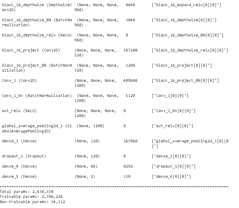

After creating the model we have to compile the model by setting up the optimizer which brings non-linearity to the model, loss functions, and the metric for scoring the model. In our case, we will be using Adam optimizer as it performs better in most of the cases. The loss function will be using binary_crossentropy as we have exactly 2 classes to classify. The metric function “accuracy” will be used to evaluate the performance of our model.

As we can see in the below code we are using callbacks. A callback is used to perform actions at various stages of training (e.g. at the start or end of an epoch, before or after a single batch, etc). 

In our case, we are using Modelcheckpoint for saving the model weights into the disk for a minimum value of validation loss. Further, we are also using ReduceLROnPlateau for reducing the learning rate of the model by a factor of 0.5 if its validation loss doesn’t improve for 2 consecutive epochs.

checkpoint = ModelCheckpoint('.mdl_wts.hdf5', monitor='val_accuracy', verbose=1, 
                             save_best_only=True, mode='max')

reduce_lr = ReduceLROnPlateau(monitor='val_loss', factor=0.5, patience=2, 
                                   verbose=1, mode='min', min_lr=0.0000001)



callbacks = [checkpoint,reduce_lr]

Model Training

In this step, we will actually train the model by fitting the model on train data and evaluating it on test data. For training the model, we are using a batch size of 32 and a number of epochs of 50.

history = model.fit(x_train,y_train,batch_size=batch_size,callbacks=callbacks, validation_data=(x_test,y_test),epochs=epochs,verbose=1)

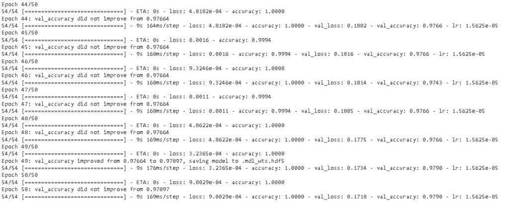
As we can see from the above training results, the model’s accuracy reached 97.90 as it reaches 50 epochs.

Model Evaluation

After training our model we will be checking the overall training history of our model.

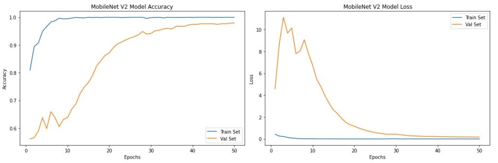
As we can see from the training history plots, the model’s validation accuracy and validation loss stabilized after 40 epochs.

Next, we will load the best weights of the model with minimum validation loss and maximum validation accuracy so that we can evaluate the performance of the model on various performance metrics.

# saving the weight of model
from keras.models import load_model
model = load_model('.mdl_wts.hdf5')

#checking the score of the model
score=model.evaluate(x_test,y_test)
print(score)

The model performed well on test data with an overall validation accuracy of 97.897%. But now we will evaluate it on completely unseen validation data so that we can assess its performance in a real sense. So for that, we have to load the validation data.

# setting the path of validation directory
M_VDIR =  "/content/drive/MyDrive/Monkey_Pox_Dataset/Val/Monkeypox/"
O_VDIR = "/content/drive/MyDrive/Monkey_Pox_Dataset/Val/Others/"

# storing all the files from directories M_VDIR and O_VDIR to MVimages and OVimages for accessing images directly
MVimages = os.listdir(M_VDIR)
OVimages = os.listdir(O_VDIR)

data=[]
labels=[]

for m in MVimages:
    try:
        image=cv2.imread(M_VDIR+m)
        image_from_array = Image.fromarray(image, 'RGB')
        size_image = image_from_array.resize((224, 224))
        data.append(np.array(size_image))
        labels.append(1)
    except AttributeError:
        print("")

for o in OVimages:
    try:
        image=cv2.imread(O_VDIR+o)
        image_from_array = Image.fromarray(image, 'RGB')
        size_image = image_from_array.resize((224, 224))
        data.append(np.array(size_image))
        labels.append(0)
    except AttributeError:
        print("")

#converting features and labels in array
feats=np.array(data)
labels=np.array(labels)

# saving features and labels for later re-use
np.save("/content/drive/My Drive/skin_cancer_dataset/feats_val",feats)
np.save("/content/drive/My Drive/skin_cancer_dataset/labels_val",labels)

# loading validation data
x_val=np.load("/content/drive/MyDrive/Monkey_Pox_Dataset/feats_val.npy")
y_val=np.load("/content/drive/MyDrive/Monkey_Pox_Dataset/labels_val.npy")

s=np.arange(x_val.shape[0])
np.random.shuffle(s)
x_val=x_val[s]
y_val=y_val[s]

# image normalization
x_val = x_val.astype('float32')/255
#one hot encoding
y_val=to_categorical(y_val,num_classes)

# checking the accuracy on valdation data
accuracy = model.evaluate(x_val, y_val, verbose=1)
print('\n', 'Validation_Accuracy:-', accuracy[1])

As we can see from the above results that validation accuracy decreased to 78.80% as we checked the model on completely unseen validation data. The reason for the decrease in accuracy may be that we have not trained some of the variations present in validation data as our training data is very small. But still, it’s a good accuracy on real-time unseen data.

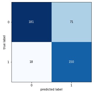
Confusion Matrix

Classification report

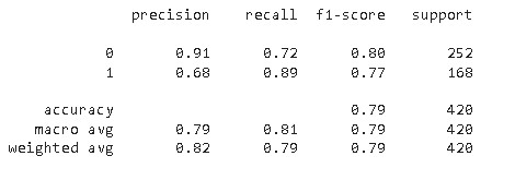
From the confusion matrix and classification report, it is evident that the model’s sensitivity is higher i.e., it is more accurate in predicting Monkeypox cases in comparison to others cases.

Sample prediction

Now we will check some of the random predictions of the model on validation data.

y_hat = model.predict(x_val)

# define text labels 
m_labels = ['MonkeyPox','Others']

# plot a random sample of test images, their predicted labels, and ground truth
fig = plt.figure(figsize=(20, 8))
for i, idx in enumerate(np.random.choice(x_val.shape[0], size=12, replace=False)):
    ax = fig.add_subplot(4,4, i+1, xticks=[], yticks=[])
    ax.imshow(np.squeeze(x_val[idx]))
    pred_idx = np.argmax(y_hat[idx])
    true_idx = np.argmax(y_val[idx])
    ax.set_title("{} ({})".format(m_labels[pred_idx], m_labels[true_idx]),
                 color=("blue" if pred_idx == true_idx else "red"))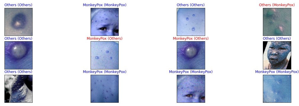

From the above code, we are populating random images from validation data and performing model predictions on those images. Every image contains a label consisting of a prediction with a true label in the bracket. The First incorrect prediction is on the first row the last image from the right where the model prediction is Others but actually it is Monkeypox whereas two more incorrect predictions are shown in the second row where the model prediction is Monkeypox but actually it is Others.

The major reason for incorrect prediction is the similarity of Monkeypox disease with other types of diseases such as Chickenpox or Measles. The effect of Monkeypox disease also differs from person to person, sometimes it may look similar to smallpox or sometimes it looks harsher than any other disease. We can improve the performance of the model by increasing our training dataset or by performing more augmentations on images in order to increase the image to make the model more robust.

The full code demonstrated in this article is available in Google Colab Notebook.

Conclusion

So, in this article, we have shown the step-wise development of a transfer learning-based MobileNet V2 model for detecting Monkeypox virus cases. Further, we have evaluated the model and found its accuracy is around 79% with higher sensitivity of 89% for Monkeypox cases. At last, we have shown the sample prediction of the model on validation data and found that in the majority of the cases, the model accurately detected Monkeypox cases whereas it fails to detect in three cases where Monkeypox infection looks too similar to other diseases.

Thank you for reading! Feel free to share your thoughts and ideas.