
Table of Contents
Social media messages are an important source of information in times of crisis. As the information on social media spreads like fire which may help recovery and disaster organizations to reach the affected place on time and provide their support services.
Twitter is one of the most popular social media platforms where people write tweets with hashtags in order to convey their message to the social media community. One of the main advantages of Twitter is that the government agencies of almost all the countries are proactive on Twitter.
Disaster Tweets Classification Challenge
As Twitter provides its tweets data for analysis through its APIs which helps research agencies/organizations to programmatically analyze tweets and recognize disasters and emergencies. This kind of alert system can help millions of people connected to the internet in the form of getting alerts in the case of an emergency or disaster. But the major challenge is how to segregate tweets conveying disaster messages from the ones which are not related to a disaster.
In this article, we will demonstrate disaster tweets classification using machine learning with a natural language processing approach. For building the machine learning model we will be using Natural Language Processing with Disaster Tweets dataset available on Kaggle competition. The dataset consists of around 10,000 tweets that were hand classified.
Dataset description
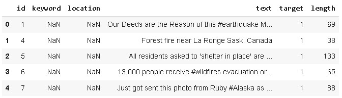
In this project, we will be using the training set of the Kaggle competition Natural Language Processing with Disaster Tweets dataset for training our machine learning models. This dataset consists of 7,613 tweets and has following features:
- id: Unique id assigned to each tweet.
- keyword: keyword associated with the tweet (although this may be blank!).
- location: The
locationtweet was sent from (may also be blank) - text: The text of a tweet.
- target: It has two values 0 denotes a normal tweet & 1 denotes an actual disaster tweet
Importing python libraries
In this step, we will import all the essential libraries required for analyzing the dataset and building the disaster tweet classification model.
# libraries for data analysis
import pandas as pd
import numpy as np
# libraries for data visualization
import seaborn as sns
import matplotlib.pyplot as plt
%matplotlib inline
# libraries for nlp task
import nltk, re, string
from string import punctuation
from nltk.corpus import stopwords
from nltk.stem import WordNetLemmatizer
from sklearn.feature_extraction.text import TfidfVectorizer
#machine learning
from sklearn.naive_bayes import MultinomialNB
from sklearn.linear_model import PassiveAggressiveClassifier
from sklearn.metrics import  accuracy_score, f1_score, precision_score,confusion_matrix, recall_score, roc_auc_score
from sklearn.model_selection import train_test_split,cross_val_score
# for importive gdrive
from google.colab import drive
drive.mount('/content/drive')
# required for nlp tasks
nltk.download('stopwords')
nltk.download('punkt')
nltk.download('wordnet')
nltk.download('omw-1.4')
Exploratory data analysis
In this step, we will analyze the dataset by extracting important information from the textual tweets feature.
Firstly, we have to check the distribution of the data.
Target distribution
sns.set_style("dark")
sns.countplot(df.target)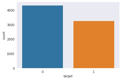
From the dataset, it is visible that the dataset has a balanced distribution of both disaster and normal tweets.
Next, we will check the length of the tweets to observe if there is any pattern present in disaster tweets in comparison to normal tweets.
# creating new column for storing length of reviews
df['length'] = df['text'].apply(len)
df.head()
Now, we will check the distribution of the newly created length column
df.length.describe()
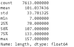
From the above statistics, we can observe that the average length of the tweets in the dataset is 101 whereas the maximum and minimum lengths are 157 and 7 respectively.
Let’s check the actual tweet having a maximum length i.e., 157
df[df['length'] == 157]['text'].iloc[0]

As we can observe from the above tweet that it’s a normal tweet and it contains more number of special characters i.e., ? which increases the length of the tweet. So cleaning the text of the tweet is also a very important step in this project.
now we can also check the actual disaster tweet having a maximum length of 151

From the above tweet, it is evident that tweet mostly contains short forms or acronyms generally popular in Twitter communication.
Now let’s compare the length of both disaster and normal tweets.
df.hist(column='length', by='target', bins=50,figsize=(10,4))
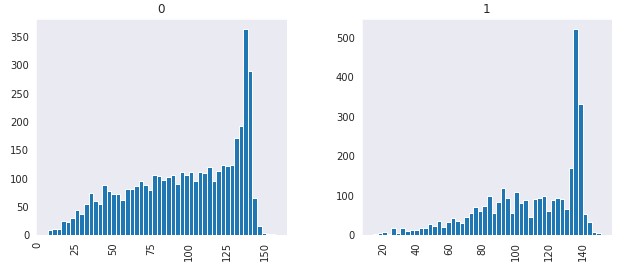
From the above distribution, it is evident that normal tweets are generally smaller in length in comparison to disaster tweets which is obvious because disaster tweets will be more explanatory in terms of explaining the type of disaster, location, and its effect.
Next, we will plot word clouds for both normal and disaster tweets to check the overall distribution of important keywords used.
For building the word cloud we have to create two subsets of the dataset consisting of only disaster and normal tweets.
# segregating dataset into disaster and normal tweets dataframe
df_1 = df[df['target']==1]
df_0 = df[df['target']==0]

stop = set(stopwords.words('english'))
punctuation = list(string.punctuation)
stop.update(punctuation)

# Removing stop words which are unneccesary from tweets text
def remove_stopwords(text):
    final_text = []
    for i in text.split():
        if i.strip().lower() not in stop:
            final_text.append(i.strip())
    return " ".join(final_text)

df_1['text']=df_1['text'].apply(remove_stopwords)
df_0['text']=df_0['text'].apply(remove_stopwords)

# plotting disaster tweets wordcloud
from wordcloud import WordCloud
plt.figure(figsize = (20,20)) # Text that is Disaster tweets
wc = WordCloud(max_words = 1000 , width = 1600 , height = 800).generate(" ".join(df_1.text))
plt.imshow(wc , interpolation = 'bilinear')

# plotting normal tweets wordcoud

plt.figure(figsize = (20,20)) # Text that is Disaster tweets
wc = WordCloud(max_words = 1000 , width = 1600 , height = 800).generate(" ".join(df_0.text))
plt.imshow(wc , interpolation = 'bilinear')
From the above wor cloud, we can observe that disaster tweets word cloud contains disaster keywords in higher frequency such as fire, death, storm, death, etc. whereas normal tweets contain usual keywords such as people, love, know, want, time, new, etc.
Data cleaning & data preparation
In this step, we will lowercase all the words, remove the stop words, tokenize the text, perform lemmatization, and remove all non-alphabetic characters from the tweet. The code for the above-mentioned task is shared below:
lemma = WordNetLemmatizer()
#creating list of possible stopwords from nltk library
stop = stopwords.words('english')

def cleanTweet(txt):
  # lowercaing
    txt = txt.lower()
    # tokenization
    words = nltk.word_tokenize(txt)
  # removing stopwords & mennatizing the words
    words = ' '.join([lemma.lemmatize(word) for word in words if word not in (stop)])
    text = "".join(words)
  # removing non-alphabetic characters
    txt = re.sub('[^a-z]',' ',text)
    return txt
#applying cleantweet function on tweet text column
df['cleaned_tweets'] = df['text'].apply(cleanTweet)
df.head()
Creating feature & target variable
In this step, we will create a feature and target variable for building a machine learning model.
y = df.target
X=df.cleaned_tweets
Train Test Split
In this step, we will divide the dataset into train and test set in the ratio of 80:20 i.e., 80% for training the machine learning model and 20% for evaluating it.
X_train, X_test, y_train, y_test = train_test_split(X, y,test_size=0.20,stratify=y, random_state=0)
TF-IDF Vectorization
In this step, we will vectorize the textual data using Term Frequency Inverse Document Frequency(TFIDF) as machine learning model only understand numeric data. Using TDIDF we will be building two variants of vectorizers: bi-grams and tri-grams. In the first case, we will be using ngram_range =(1,2) which means it will take both unigram and bi-grams as a feature from text whereas in the second case we will use ngram_range =(1,3) i.e., unigram,bi-grams, and tri-grams as a feature.
# bigrams
tfidf_vectorizer = TfidfVectorizer(stop_words='english', max_df=0.8, ngram_range=(1,2))
tfidf_train_2 = tfidf_vectorizer.fit_transform(X_train)
tfidf_test_2 = tfidf_vectorizer.transform(X_test)

# trigrams
tfidf_vectorizer_3 = TfidfVectorizer(stop_words='english', max_df=0.8, ngram_range=(1,3))
tfidf_train_3 = tfidf_vectorizer_3.fit_transform(X_train)
tfidf_test_3 = tfidf_vectorizer_3.transform(X_test)
Building machine learning model
In this step, we will fit machine learning models i.e., Multinomial Naive Bayes and Passive Aggressive Classifier to the TF-IDF vectorized data.
## Multi nomial Naive Bayes - bigram
mnb_tf_bigram = MultinomialNB()
mnb_tf_bigram .fit(tfidf_train_2, y_train)

# Passive Aggressive Classifier -bigram
pass_tf_bigram = PassiveAggressiveClassifier()
pass_tf_bigram.fit(tfidf_train_2, y_train)

## Multi nomial Naive Bayes - trigram
mnb_tf_trigram = MultinomialNB()
mnb_tf_trigram .fit(tfidf_train_3, y_train)

# Passive Aggressive Classifier -trigram
pass_tf_trigram = PassiveAggressiveClassifier()
pass_tf_trigram.fit(tfidf_train_3, y_train)
After fitting the model into a training set, now we will proceed toward cross-validation.
Cross-validation
In this step, we will cross-validate both the machine learning models on bi-gram and tri-gram variants of TFIDF vectorizer-based training data.
kfold = model_selection.KFold(n_splits=10)
scoring = 'accuracy'
acc_mnb2 = cross_val_score(estimator = mnb_tf_bigram, X = tfidf_train_2, y = y_train, cv = kfold,scoring=scoring)
acc_passtf2 = cross_val_score(estimator = pass_tf_bigram, X = tfidf_train_2, y = y_train, cv = kfold,scoring=scoring)
acc_mnb3 = cross_val_score(estimator = mnb_tf_trigram, X = tfidf_train_3, y = y_train, cv = kfold,scoring=scoring)
acc_passtf3 = cross_val_score(estimator = pass_tf_trigram, X = tfidf_train_3, y = y_train, cv = kfold,scoring=scoring)
# compare the average 10-fold cross-validation accuracy
crossdict = {
'MNB-Bigram': acc_mnb2.mean(),
'PassiveAggressive-Bigram':acc_passtf2.mean(),
'MNB-Trigram': acc_mnb3.mean(),
'PassiveAggressive-Trigram': acc_passtf3.mean() }
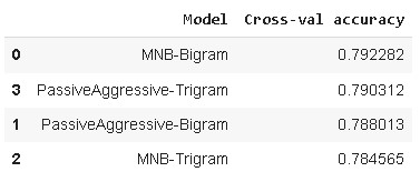
cross_df = pd.DataFrame(crossdict.items(), columns=['Model', 'Cross-val accuracy'])
cross_df = cross_df.sort_values(by=['Cross-val accuracy'], ascending=False)
cross_df
Model Evaluation
In this step, we will evaluate both the machine learning models on the test set based on different performance metrics such as accuracy, precision, sensitivity(recall), f1-score, and roc value.
Firstly, we will evaluate our base model i.e., Multinomial Naive Bayes fitted on TFIDF Bigram, and later compare its performance with other models.
pred_mnb2 = mnb_tf_bigram.predict(tfidf_test_2)

acc= accuracy_score(y_test, pred_mnb2)

prec = precision_score(y_test, pred_mnb2)
rec = recall_score(y_test, pred_mnb2)
f1 = f1_score(y_test, pred_mnb2)
roc=roc_auc_score(y_test, pred_mnb2)

model_results =pd.DataFrame([['Multinomial Naive Bayes-Bigram',acc, prec,rec,f1,roc]],
               columns = ['Model', 'Accuracy','Precision', 'Sensitivity', 'F1 Score','ROC'])

model_results
Comparison with other models
y_pred_passtf2 = pass_tf_bigram.predict(tfidf_test_2)
y_pred_mnb3 = mnb_tf_trigram.predict(tfidf_test_3)
y_pred_passtf3 =pass_tf_trigram.predict(tfidf_test_3)


models = {
                'PassiveAggressive-Bigram':y_pred_passtf2,

                'MNB-Trigram': y_pred_mnb3,

                'PassiveAggressive-Trigram': y_pred_passtf3 }

models = pd.DataFrame(models)

for column in models:

    acc= accuracy_score(y_test, models[column])
    roc=roc_auc_score(y_test, models[column])
    prec = precision_score(y_test, models[column])
    rec = recall_score(y_test, models[column])
    f1 = f1_score(y_test, models[column])


    results =pd.DataFrame([[column,acc, prec,rec,f1,roc]],
               columns = ['Model', 'Accuracy','Precision', 'Sensitivity', 'F1 Score','ROC'])
    model_results = model_results.append(results, ignore_index = True)

# function to highlight maximum value of numeric columns
def highlight_max(s):
    if s.dtype == np.object:
        is_max = [False for _ in range(s.shape[0])]
    else:
        is_max = s == s.max()
    return ['background: lightgreen' if cell else '' for cell in is_max]

model_results.style.apply(highlight_max)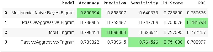
From the above results, it is evident that Multinomial Naive Bayes -Bigram accuracy is highest i.e., 80.039% whereas sensitivity and F1-score are highest for Passive Aggressive Classifier -Trigram i.e., 76.45% and 75.18% respectively.
The need for this project is to accurately detect more number of disaster cases so recall i.e., higher sensitivity of the model is important. Hence, the best model for this use case would be the Passive Aggressive Classifier -Trigram
Most Informative features
In this step, we will find out the most important features based on our selected model i.e., Passive Aggressive Classifier -Trigram. The code for the same is shared below.
def most_informative_feature_for_binary_classification(vectorizer, classifier, n=100):
    """
    See: https://stackoverflow.com/a/26980472

    Identify most important features if given a vectorizer and binary classifier. Set n to the number
    of weighted features you would like to show. (Note: current implementation merely prints and does not
    return top classes.)
    """

    class_labels = classifier.classes_
    feature_names = vectorizer.get_feature_names_out()
    topn_class1 = sorted(zip(classifier.coef_[0], feature_names))[:n]
    topn_class2 = sorted(zip(classifier.coef_[0], feature_names))[-n:]

    for coef, feat in topn_class1:
        print(class_labels[0], coef, feat)

    print()

    for coef, feat in reversed(topn_class2):
        print(class_labels[1], coef, feat)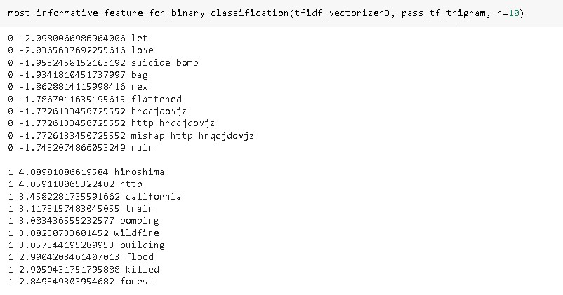
As we can see from the above results the model has accurately selected relevant keywords in case of disaster tweets such as wildfire, bombing, flood, killed, etc.
Sample prediction
In this step, we will use our best model to predict sample tweets for checking the overall validity of the model.
sentences = [
  "Just happened a terrible car crash",
    "Heard about #earthquake is different cities, stay safe everyone.",
    "No I don't like cold!",
    "@RosieGray Now in all sincerety do you think the UN would move to Israel if there was a fraction of a chance of being annihilated?"
  ]

tfidf_trigram = tfidf_vectorizer3.transform(sentences)


predictions = pass_tf_trigram.predict(tfidf_trigram)

for text, label in zip(sentences, predictions):
    if label==1:
        target="Disaster Tweet"
        print("text:", text, "\nClass:", target)
        print()
    else:
        target="Normal Tweet"
        print("text:", text, "\nClass:", target)
        print()
As per the prediction results, we can see that model has accurately detected the first two tweets as disaster tweets while the next two tweets as normal tweets which signifies that the model is trained to classify disaster and normal tweets on real-time data.
Conclusion
In this article, we have demonstrated the training of a machine learning model using natural language processing for detecting disaster tweets from the Twitter dataset. Further, we have demonstrated different data pre-processing techniques for cleaning the data. In the end, we have trained two machine learning models i.e., Multinomial Naive Bayes and Passive Aggressive Classifier on Bi-gram and Tr-gram variants of TFIDF vectorized data and found Passive Aggressive Classifier trained on Trigram performed best for this use-case. Lastly, we have also extracted important features of the model for both disaster and normal tweets classes and performed predictions on sample test sentences to check the overall performance of the model.
Thank you for reading! Feel free to share your thoughts and ideas.