
Table of Contents
Diabetes mellitus is a metabolic chronic disease where blood sugar (glucose) levels remain higher than normal levels in the human body. According to the International Diabetes Federation, the total number of people suffering from diabetes will rise to 643 million by 2030 and a further 783 million by 2045. The total number of casualties happened due to diabetes so far is 6.7 million which signifies the seriousness of this disease.
Some of the common factors responsible for diabetes are family history, physical inactivity due to work pressure, mode of working (work from home and hybrid mode of working), high fat diet, cheap and unhealthy junk foods intake, high alcohol intake.

The main reason which is responsible for increasing rate of disease is the human lifestyle. Today many people including young adults and even children below 10 years are very much prone to eat cheap and unhealthy junk food. As a result of this, obesity has become an epidemic and obesity is one of the contributing factors to diabetes.
Another important factor in diabetes is physical inactivity due to a busy work schedule and mode of working. Due to the ongoing pandemic COVID-19, companies changed their mode of working i.e., shifted to work from home, and hybrid mode of working resulting in lesser physical movement and constant sitting for long hours which is also a contributing factor to developing diabetes.

With current living patterns and standard of living, diabetes is pretty common in people’s daily life, and its increasing at an alarming rate. So, in order to control it, its early diagnosis is very important.
Therefore, in this post, we will demonstrate how we can apply machine learning techniques for detecting diabetes in its early stages. For this task, we have used the Early-stage diabetes risk prediction dataset available on the UCI Machine Learning repository. This has been collected using direct questionnaires from the patients of Sylhet Diabetes Hospital in Sylhet, Bangladesh, and approved by a doctor. This is a symptomatic dataset containing the symptoms of newly diabetic or would-be diabetic patients.
The datasets consist of 16 medical predictor variables and one target variable, class. The details of features in the dataset are given below:
| S.No. | Feature | Data Type |
| 1. | Age | Numeric |
| 2. | Sex (Male/Female) | String |
| 3. | Polyuria (Yes/No) | String |
| 4. | Polydipsia (Yes/No) | String |
| 5. | sudden weight loss (Yes/No) | String |
| 6. | weakness (Yes/No) | String |
| 7. | Polyphagia (Yes/No) | String |
| 8. | Genital thrush (Yes/No) | String |
| 9. | visual blurring (Yes/No) | String |
| 10. | Itching (Yes/No) | String |
| 11. | Irritability (Yes/No) | String |
| 12. | delayed healing (Yes/No) | String |
| 13. | partial paresis (Yes/No) | String |
| 14. | muscle stiffness (Yes/No) | String |
| 15. | Alopecia (Yes/No) | String |
| 16. | Obesity (Yes/No) | String |
| 17. | Class (Positive/Negative) | String |
So, before jumping on to python code for dataset analysis and model building we should have the following python libraries installed in our machine or in our virtual environment.
Installations:
This project requires Python 3.x and the following Python libraries should be installed to get the project started:
We also recommend installing Anaconda, a pre-packaged Python distribution that contains all of the necessary libraries and software for this project which also includes a Jupiter notebook to run and execute the IPython Notebook.
Importing Libraries
So, after installing all the important libraries in python, we have to import them so that we can utilize them as soon as we need them.
import warnings
warnings.filterwarnings('ignore')
import numpy as np
import pandas as pd
from sklearn.preprocessing import MinMaxScaler
from sklearn.model_selection import train_test_split,cross_val_score
from sklearn.linear_model import LogisticRegression
from sklearn.metrics import accuracy_score, f1_score, precision_score,confusion_matrix, recall_score, roc_auc_score
from xgboost import XGBClassifier
from sklearn.ensemble import RandomForestClassifier,AdaBoostClassifier
from sklearn.svm import SVC
import matplotlib.pyplot as plt
%matplotlib inline
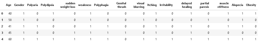
from IPython.display import ImageAfter importing the dataset, we have to see the first look at the dataset that we will be using for building the diabetes detection model. So, for that, we have to read the dataset using the pandas library in python as given below.
#reading the dataset
df = pd.read_csv('diabetes_data_upload.csv')

#showing first few rows of the dataset
df.head()
Checking Missing Values
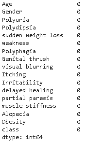
The next step is to check the missing values in the dataset. For doing so we have to run the below code which will help in visualizing missing values per feature.
#checking missing values per feature
df.isna().sum()
Exploratory Data Analysis
In this step, we will explore all the features and their distribution to understand the underlying pattern in the dataset with respect to each class of the target variable. So, to start with we will first explore the target variable i.e., class.
1. Distribution of target variable
This step is very important because it will help in understanding whether the dataset is balanced or unbalanced i.e., whether one class value is too much lesser in percentage <10% in comparison to other class value. This state is known as the dataset imbalance issue. So, for checking the same we have executed the below code.
# plotting to create pie chart and bar plot distribution of target variable
plt.figure(figsize=(14,7))
plt.subplot(121)
df["class"].value_counts().plot.pie(autopct = "%1.0f%%",colors = sns.color_palette("prism",7),startangle = 60,labels=["Positive","Negative"],
wedgeprops={"linewidth":2,"edgecolor":"k"},explode=[.1,0],shadow =True)
plt.title("Distribution of Target  variable")

plt.subplot(122)
ax = df["class"].value_counts().plot(kind="barh")

for i,j in enumerate(df["class"].value_counts().values):
    ax.text(.7,i,j,weight = "bold",fontsize=20)

plt.title("Count of Traget variable")
plt.show()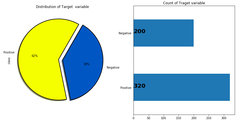
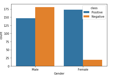
2. Distribution of Gender
In this step, we have checked the distribution of the Gender feature which is a binary feature having two values only i.e., Male / Female. The code for checking the distribution is given below:
#plotting barchart for distribution
sns.countplot(df['Gender'],hue=df['class'], data=df)
#plotting target variable wrt Gender variable
plot_criteria= ['Gender', 'class']
cm = sns.light_palette("red", as_cmap=True)
(round(pd.crosstab(df[plot_criteria[0]], df[plot_criteria[1]], normalize='columns') * 100,2)).style.background_gradient(cmap = cm)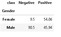
From the above distribution of gender, it is evident that Males have a higher distribution of negative diabetes in comparison to females who have merely 9.5% of negative diabetes cases. So, we can say that the dataset is somewhat biased towards the male side.
3. Distribution of Polyuria
Polyuria is a medical condition where adults have a very frequent passage of large volumes of urine i.e., > 3 liters a day whereas the normal range is 1 to 2 liters a day.
The most common cause of polyuria in both adults and children is uncontrolled diabetes mellitus, resulting in osmotic diuresis which develops when glucose levels are so high that glucose is excreted in the urine resulting in a large volume of urine output.
#plotting target variable wrt Polyuria variable
plot_criteria= ['Polyuria', 'class']
cm = sns.light_palette("red", as_cmap=True)
(round(pd.crosstab(df[plot_criteria[0]], df[plot_criteria[1]], normalize='columns') * 100,2)).style.background_gradient(cmap = cm)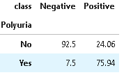
From the above distribution, it is clear that the presence of Polyuria signifies strong chances of diabetes in comparison to its absence.
4. Distribution of Polydipsia
Polydipsia is defined as a medical condition of being thirsty all the time. It is also usually accompanied by temporary or prolonged dryness of the mouth. It is one of the initial signs of diabetes.
#plotting target variable wrt Polydispia variable
plot_criteria= ['Polydipsia', 'class']
cm = sns.light_palette("red", as_cmap=True)
(round(pd.crosstab(df[plot_criteria[0]], df[plot_criteria[1]], normalize='columns') * 100,2)).style.background_gradient(cmap = cm)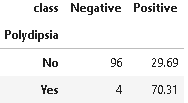
From the above distribution, it is clear that the presence of Polydipsia signifies strong chances of diabetes in comparison to its absence.
5. Distribution of sudden weight loss
If there is a sudden weight loss without any reason then this may also be a sign of diabetes.
#plotting target variable wrt sudden weight loss variable
plot_criteria= ['sudden weight loss', 'class']
cm = sns.light_palette("red", as_cmap=True)
(round(pd.crosstab(df[plot_criteria[0]], df[plot_criteria[1]], normalize='columns') * 100,2)).style.background_gradient(cmap = cm)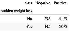
From the above distribution, it is evident that patients having sudden weight loss are more prone to diabetes
6. Distribution of Weakness
plot_criteria= ['weakness', 'class']
cm = sns.light_palette("red", as_cmap=True)
(round(pd.crosstab(df[plot_criteria[0]], df[plot_criteria[1]], normalize='columns') * 100,2)).style.background_gradient(cmap = cm)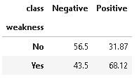
7. Distribution of Polyphagia
Polyphagia is a medical condition of extreme hunger where hunger won’t go away even after eating more food.
plot_criteria= ['Polyphagia', 'class']
cm = sns.light_palette("red", as_cmap=True)
(round(pd.crosstab(df[plot_criteria[0]], df[plot_criteria[1]], normalize='columns') * 100,2)).style.background_gradient(cmap = cm)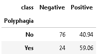
The above distribution suggests that polyphagia is an important contributor to diabetes.
8. Distribution of genital thrush
Genital Thrush also known as candidiasis is a common medical condition caused by a type of yeast/bacteria called Candida. It mainly affects the vagina, though it may affect the penis too, and is very irritating and painful.
plot_criteria= ['Genital thrush', 'class']
cm = sns.light_palette("red", as_cmap=True)
(round(pd.crosstab(df[plot_criteria[0]], df[plot_criteria[1]], normalize='columns') * 100,2)).style.background_gradient(cmap = cm)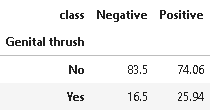
From the above distribution, it is not clear whether genital thrush has any correlation with diabetes or not.
9. Distribution of visual blurring
plot_criteria= ['visual blurring', 'class']
cm = sns.light_palette("red", as_cmap=True)
(round(pd.crosstab(df[plot_criteria[0]], df[plot_criteria[1]], normalize='columns') * 100,2)).style.background_gradient(cmap = cm)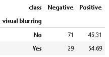
10. Distribution of Itching
Itching is a common condition and it may or may not be a contributing factor and the same is evident from the below distribution. But itching combined with other medical conditions may be a potential sign of diabetes.
plot_criteria= ['Itching', 'class']
cm = sns.light_palette("red", as_cmap=True)
(round(pd.crosstab(df[plot_criteria[0]], df[plot_criteria[1]], normalize='columns') * 100,2)).style.background_gradient(cmap = cm)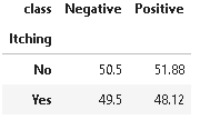
11. Distribution of Irritability
plot_criteria= ['Irritability', 'class']
cm = sns.light_palette("red", as_cmap=True)
(round(pd.crosstab(df[plot_criteria[0]], df[plot_criteria[1]], normalize='columns') * 100,2)).style.background_gradient(cmap = cm)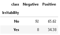
12. Distribution of Delayed Healing
Diabetes can cause wounds to heal slowly, increasing the risk of infections and other severe complications.
plot_criteria= ['delayed healing', 'class']
cm = sns.light_palette("red", as_cmap=True)
(round(pd.crosstab(df[plot_criteria[0]], df[plot_criteria[1]], normalize='columns') * 100,2)).style.background_gradient(cmap = cm)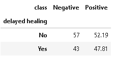
13. Distribution of Partial Paresis
Paresis involves loosening the strength of a muscle or group of muscles. It may also be referred to as partial or mild paralysis. Unlike paralysis, people with paresis can still move their muscles. These movements are just too weaker than normal.
plot_criteria= ['partial paresis', 'class']
cm = sns.light_palette("red", as_cmap=True)
(round(pd.crosstab(df[plot_criteria[0]], df[plot_criteria[1]], normalize='columns') * 100,2)).style.background_gradient(cmap = cm)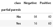
The above distribution suggests that partial paresis is an important symptom in diabetes.
14. Distribution of Muscle Stiffness
plot_criteria= ['muscle stiffness', 'class']
cm = sns.light_palette("red", as_cmap=True)
(round(pd.crosstab(df[plot_criteria[0]], df[plot_criteria[1]], normalize='columns') * 100,2)).style.background_gradient(cmap = cm)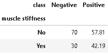
15. Distribution of Obesity
plot_criteria= ['Obesity', 'class']
cm = sns.light_palette("red", as_cmap=True)
(round(pd.crosstab(df[plot_criteria[0]], df[plot_criteria[1]], normalize='columns') * 100,2)).style.background_gradient(cmap = cm)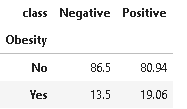
From the above distribution, it is evident that the dataset has very less obese patients but in general, we all know that obesity is more positively correlated with diabetes.
16. Alopecia
Alopecia areata is a medical condition of sudden hair loss that starts with one or more circular bald patches that may overlap. The main symptom is hair loss.
plot_criteria= ['Alopecia', 'class']
cm = sns.light_palette("red", as_cmap=True)
(round(pd.crosstab(df[plot_criteria[0]], df[plot_criteria[1]], normalize='columns') * 100,2)).style.background_gradient(cmap = cm)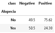
Data Pre-processing
In this step, we have to pre-process the target variable and other input features in order to prepare them for model building.
As the target variable consists of string values i.e., Positive and Negative we have to convert it into numerical format i.e., 1, 0. Below is the code for transforming the target variable into the numerical format.
# transforming target column from string to numeric format
df['class'] = df['class'].apply(lambda x: 0 if x=='Negative' else 1)
Next, we have to create features and target variables so we have to segregate all the features excluding target variables as input features i.e., X whereas the target variable class will be assigned as Y which we have to predict.
# creating feature and target variable
X= df.drop(['class'],axis=1)
y=df['class']
Now, we have to convert all the features containing string values into the numerical format and for doing so we have to use Label Encoder. Label Encoder is a method for encoding categorical values into the numerical format.
#creating a list of object datatypes

objList = X.select_dtypes(include = "object").columns

#Label Encoding for object to numeric conversion
from sklearn.preprocessing import LabelEncoder
le = LabelEncoder()

for feat in objList:
    X[feat] = le.fit_transform(X[feat].astype(str))

print (X.info())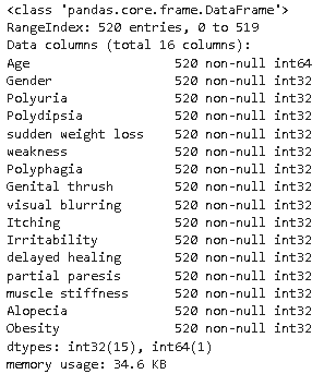
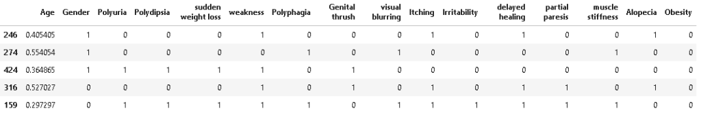
As we can see from the above output, all the input features are now converted to numeric int32 format. Now let’s take a look at the dataset.
Correlation
In this step, we will see which features are more correlated with target variables.
For checking the correlation of all input features with the target variable in the tabular format we need to execute the below code.
# calculating correlation of all the input variables with target variable
X.corrwith(y)
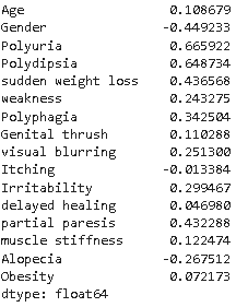
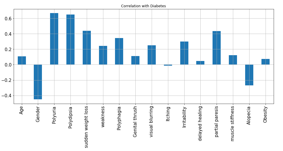
From the above graph, it is evident that Polyuria and Polydipsia are the most positively correlated features with respect to diabetes whereas Gender and Alopecia are the negatively correlated features.
Train Test Split
In this step, we have to split the dataset into training and test sets but with an equal proportion of both the classes in both the training and test set. For achieving the same we have to specify stratify argument as y so that it split the dataset into an equal proportion of classes.
# train test split
X_train, X_test, y_train, y_test = train_test_split(X, y, test_size = 0.2,stratify=y, random_state = 1234)

## checking distribution of traget variable in train test split
print('Distribution of traget variable in training set')
print(y_train.value_counts())

print('Distribution of traget variable in test set')
print(y_test.value_counts())
Data Normalization
In this dataset, we have only one numeric feature i.e., Age whose values are inconsistent in terms of magnitude in comparison to all other features. So we have to normalize it on the same scale so that the machine learning model will converge easily and will give consistent prediction without data bias.
# instantiating minmax scaling object
minmax = MinMaxScaler()
#apply minmax scaling on Age feature
X_train[['Age']] = minmax.fit_transform(X_train[['Age']])
X_test[['Age']] = minmax.transform(X_test[['Age']])

X_train.head()
Model Building
This is the most awaited step in which we actually build machine learning models for predicting diabetes cases. So, firstly we will build a Logistic Regression model which is a linear and most basic model, and further, we will compare its performance with the Random forest model.
1. Logistic Regression (Base Model)
Logistic regression is a statistical method for modeling probabilities for classification problems with binary outcomes. Its an extension of linear regression which is generally used for modeling continuous values.
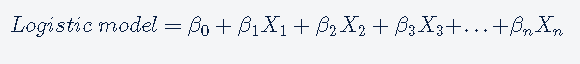
The logistic regression is based on logistic function. the logistic function is defined as follows:

The values of a logistic function will range from 0 to 1. The values of Z will vary from −∞ to +∞.
Logistic regression is a very popular and most basic machine learning algorithm for binary classification tasks because it can convert the values of logits (log-odds), which can range from −∞ to +∞ to a range between 0 and 1. As logistic functions output the probability of occurrence of an event, it can be applied to many real-life scenarios. Another important reason for its popularity is that it can handle categorical variables.
The logistic model outputs the logits, i.e. log-odds; and the logistic function outputs the probabilities.

The output of the Logistic function will be the probabilities
Logistic regression is available as a python library available under sklearn
from sklearn.linear_model import LogisticRegression
logi = LogisticRegression(random_state = 0, penalty = 'l2')
logi.fit(X_train, y_train)
As we can see from the above code, we have used only the default parameters of the Logistic regression algorithm.
10-Fold Cross-Validation
from sklearn import model_selection

kfold = model_selection.KFold(n_splits=10, random_state=7)
scoring = 'accuracy'

acc_logi = cross_val_score(estimator = logi, X = X_train, y = y_train, cv = kfold,scoring=scoring)
acc_logi.mean()
Model Evaluation
In this step, we will evaluate the logistic regression model on the test set.
y_predict_logi = logi.predict(X_test)
acc= accuracy_score(y_test, y_predict_logi)
roc=roc_auc_score(y_test, y_predict_logi)
prec = precision_score(y_test, y_predict_logi)
rec = recall_score(y_test, y_predict_logi)
f1 = f1_score(y_test, y_predict_logi)

results = pd.DataFrame([['Logistic Regression',acc, acc_logi.mean(),prec,rec, f1,roc]],
               columns = ['Model', 'Accuracy','Cross Val Accuracy', 'Precision', 'Recall', 'F1 Score','ROC'])
results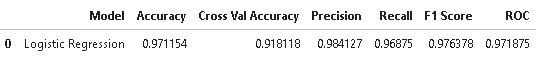
Plotting Confusion Matrix
cm_logi = confusion_matrix(y_test, y_predict_logi)
plt.title('Confusion matrix of the Logistic classifier')
sns.heatmap(cm_logi,annot=True,fmt="d")
plt.show()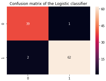
From the above results, it is evident that Logistic regression has done a pretty good job in identifying diabetic cases. Next, we will plot important features which are contributing to predicting diabetes.
Plotting Feature Importance – Logistic Regression
#plotting feature importance
feature_importance = abs(logi.coef_[0])
feature_importance = 100.0 * (feature_importance / feature_importance.max())
sorted_idx = np.argsort(feature_importance)
pos = np.arange(sorted_idx.shape[0]) + .3

featfig = plt.figure(figsize=(12,8))
featax = featfig.add_subplot(1, 1, 1)
featax.barh(pos, feature_importance[sorted_idx], align='center')
featax.set_yticks(pos)
featax.set_yticklabels(np.array(X_train.columns)[sorted_idx], fontsize=8)
featax.set_xlabel('Relative Feature Importance')

plt.tight_layout()
plt.show()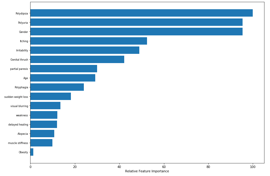
So, based on the above plot, the top 5 most contributing features of the logistic regression model are Polydipsia, Polyuria, Gender, Itching, and Irritability.
2. Random Forest
Next, we will build a more advanced tree-based model i.e., a Random forest. The random forest algorithm is based on the bagging ensemble technique which mostly works well as it combines the power of multiple decision trees. The other important reason for selecting random forest in this use case is feature selection as it also supports feature selection by giving feature importance.
Random forest is defined under the ensemble method in sklearn library.
from sklearn.ensemble import RandomForestClassifier

rf = RandomForestClassifier(criterion='gini',n_estimators=100)
rf.fit(X_train,y_train)
For this iteration, we have used 100 trees and Gini as the criterion for building trees.
Cross-Validation
kfold = model_selection.KFold(n_splits=10, random_state=7)
scoring = 'accuracy'

acc_rf = cross_val_score(estimator = rf, X = X_train, y = y_train, cv = kfold,scoring=scoring)
acc_rf.mean()
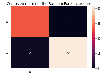
Model Evaluation
In this step, we have evaluated the random forest model on the test set and compared it with the performance of the logistic regression model.
y_predict_r = rf.predict(X_test)
roc=roc_auc_score(y_test, y_predict_r)
acc = accuracy_score(y_test, y_predict_r)
prec = precision_score(y_test, y_predict_r)
rec = recall_score(y_test, y_predict_r)
f1 = f1_score(y_test, y_predict_r)

model_results = pd.DataFrame([['Random Forest (Untuned)',acc, acc_rf.mean(),prec,rec, f1,roc]],
               columns = ['Model', 'Accuracy','Cross Val Accuracy', 'Precision', 'Recall', 'F1 Score','ROC'])
results = results.append(model_results, ignore_index = True)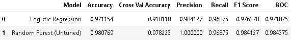
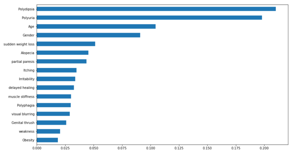
Plotting Feature Importance – Random Forest
feat_importances = pd.Series(rf.feature_importances_, index=X_train.columns)
feat_importances.sort_values().plot(kind="barh",figsize=(14, 8))
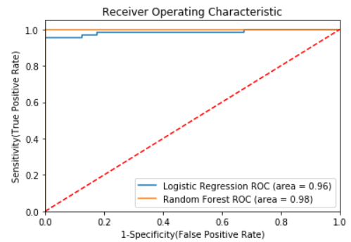
From the above results, it is evident that random forest performed better on this dataset with higher precision, accuracy, f1-score, and ROC values.
Plotting ROC AUC
In this step, we will plot the ROC curve for both Logistic regression and the Random forest algorithm to see which algorithm performed better in terms of detecting diabetes cases.
Conclusion
In this post, we have discussed the seriousness of diabetes disease and its emergence to detect it in early-stage for controlling the death rates globally. We have demonstrated the exploratory data analysis by analyzing different features in the dataset. Further, we have performed necessary data preprocessing and applied logistic regression and random forest machine learning algorithms and compared their performance, and found that random forest performed better in terms of accuracy, precision, f1-score, and ROC values. Further, we have analyzed important features contributing to the prediction of diabetes cases and found that the top 5 most contributing features are Polydipsia, Polyuria, Age, Gender, and sudden weight loss. Further, you can also perform feature selection by selecting the 10 most important features using random forest feature importance and checking how much performance degrades in the case of logistic regression and random forest model.
We hope that this post will help you in understanding the real-time healthcare problem of diabetes detection and the implementation of its solution by applying machine learning.
You can also refer to this video on diabetes detection which is available on our channel Wisdom ML on YouTube. Apart from that full code demonstrated in this post is available at the Git repo.
Enjoy Happy Learning. !!!!!