
Table of Contents
What is Heart disease ?
Heart disease develops when arteries supplying blood to the heart get blocked with plague. The plague consists of cholesterol and other substances which causes the arteries to become hardened and narrow. As a result of this, the heart receives lesser blood and oxygen supply resulting in stroke or heart attack.
Heart disease, also known as cardiovascular disease (CVD) is one of the deadliest diseases in the world. According to WHO, 17.9 million people die each year from heart disease, which is approximately 32% of all the casualties globally.

Statistics of Heart Disease in US
The Heart Disease and Stroke Statistics—2019 Update from the American Heart Association indicate that:
- Heart Disease (including Coronary Heart Disease, Hypertension, and Stroke) remains the No. 1 cause of death accounting for 874,613 deaths in the US.
- Approximately every 40 seconds, someone in the United States will have a myocardial infarction.
- In 2019, stroke accounted for approximately 1 of every 19 deaths in the United States.
- On average in 2019, someone died of a stroke every 3 minutes 30 seconds in the United States
CVD claims more lives each year in the United States than all forms of cancer and Chronic Lower Respiratory Disease (CLRD) combined. From 2017 to 2018, the average annual expenditure on heart disease was $228.7 billion in the United States.
From the above statistical data, it is evident that heart disease is a very serious disease but if it gets diagnosed at an early stage, we can reduce the number of deaths significantly. So, in this article, we will demonstrate how we can build an early-stage heart disease prediction model using machine learning in python which will help cardiologists in identifying early-stage potential heart disease cases.
Dataset description
In this project, we have used Heart Disease Dataset (Comprehensive) available on Kaggle. This dataset comprises 11 features and a target variable. It has 6 nominal variables and 5 numeric variables. The detailed description of all the features is as follows:
1. Age: Patients Age in years (Numeric)
2. Sex: Gender of patient (Male – 1, Female – 0) (Nominal)
3. Chest Pain Type: Type of chest pain experienced by patient categorized into 1 typical, 2 typical angina, 3 non-anginal pain, 4 asymptomatic (Nominal)
4. resting bp s: Level of blood pressure at resting mode in mm/HG (Numerical)
5. cholesterol: Serum cholesterol in mg/dl (Numeric)
6. fasting blood sugar: Blood sugar levels on fasting > 120 mg/dl represents 1 in case of true and 0 as false (Nominal)
7. resting ecg: Result of an electrocardiogram while at rest are represented in 3 distinct values 0 : Normal 1: Abnormality in ST-T wave 2: Left ventricular hypertrophy (Nominal)
8. max heart rate: Maximum heart rate achieved (Numeric)
9. exercise angina: Angina induced by exercise 0 depicting NO 1 depicting Yes (Nominal)
10. oldpeak: Exercise-induced ST-depression in comparison with the state of rest (Numeric)
11. ST slope: ST-segment measured in terms of the slope during peak exercise 0: Normal 1: Upsloping 2: Flat 3: Downsloping (Nominal)
Target variable
12. target: It is the target variable that we have to predict 1 means the patient is suffering from heart risk and 0 means the patient is normal.
Required Libraries
This project requires Python 3.8 and the following Python libraries should be installed to get the project started:
We also recommend installing Anaconda, a pre-packaged Python distribution that contains all of the necessary libraries and software for this project which also includes Jupiter notebook to run and execute the IPython Notebook.
Importing Libraries
# data wrangling & pre-processing
import pandas as pd
import numpy as np

# data visualization
import matplotlib.pyplot as plt
%matplotlib inline
import seaborn as sns

from sklearn.model_selection import train_test_split

#model validation
from sklearn.metrics import log_loss,roc_auc_score,precision_score,f1_score,recall_score,roc_curve,auc
from sklearn.metrics import classification_report, confusion_matrix,accuracy_score,fbeta_score,matthews_corrcoef
from sklearn import metrics

# cross validation
from sklearn.model_selection import StratifiedKFold

# machine learning algorithms
from sklearn.linear_model import LogisticRegression
from sklearn.ensemble import RandomForestClassifier,VotingClassifier,AdaBoostClassifier,GradientBoostingClassifier,RandomForestClassifier,ExtraTreesClassifier
from sklearn.neural_network import MLPClassifier
from sklearn.tree import DecisionTreeClassifier
from sklearn.linear_model import SGDClassifier
from sklearn.discriminant_analysis import LinearDiscriminantAnalysis
from sklearn.neighbors import KNeighborsClassifier
from sklearn.naive_bayes import GaussianNB
from sklearn.svm import SVC
import xgboost as xgb

from scipy import stats
After importing the necessary libraries shown above we will proceed to load the dataset.
Loading Dataset
# reading heart disease dataset
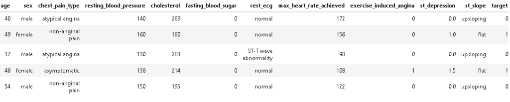
dt = pd.read_csv('heart_statlog_cleveland_hungary_final.csv')As we have read the dataset, let’s see some of the sample records in the dataset.
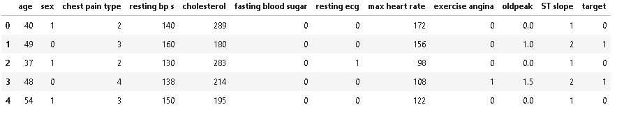
As we can see from the above dataset entries, some of the features should be nominal and be encoded as their category type. In the next step, we will encode features to their respective category as per the dataset description.
Data Cleaning & Preprocessing
As we have seen in the dataset, the name of the features have weird naming patterns with spaces which will create issues during the analysis phase, so first, we will change the name of those features into a standard format and then we will encode the features into categorical variables.
# renaming features to proper name
dt.columns = ['age', 'sex', 'chest_pain_type', 'resting_blood_pressure', 'cholesterol', 'fasting_blood_sugar',
               'rest_ecg', 'max_heart_rate_achieved','exercise_induced_angina', 'st_depression',
               'st_slope','target']
# converting features to categorical features dt['chest_pain_type'][dt['chest_pain_type'] == 1] = 'typical angina' dt['chest_pain_type'][dt['chest_pain_type'] == 2] = 'atypical angina' dt['chest_pain_type'][dt['chest_pain_type'] == 3] = 'non-anginal pain' dt['chest_pain_type'][dt['chest_pain_type'] == 4] = 'asymptomatic' dt['rest_ecg'][dt['rest_ecg'] == 0] = 'normal' dt['rest_ecg'][dt['rest_ecg'] == 1] = 'ST-T wave abnormality' dt['rest_ecg'][dt['rest_ecg'] == 2] = 'left ventricular hypertrophy' dt['st_slope'][dt['st_slope'] == 1] = 'upsloping' dt['st_slope'][dt['st_slope'] == 2] = 'flat' dt['st_slope'][dt['st_slope'] == 3] = 'downsloping' dt["sex"] = dt.sex.apply(lambda x:'male' if x==1 else 'female')
Checking the distribution of categorical variables
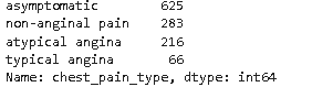
dt['chest_pain_type'].value_counts()
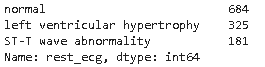
dt['rest_ecg'].value_counts()
dt['st_slope'].value_counts()
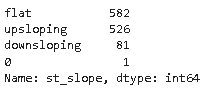
As we can see from the above distribution of st_slope, the value 0 has only 1 record and the 0 value also has no description in the dataset description. So we will remove the record having a st_slope value of 0.
#dropping row with st_slope =0
dt.drop(dt[dt.st_slope ==0].index, inplace=True)
Now as we have done feature encoding let’s have a look at the dataset.
As we can see features are encoded successfully to their respective categories. Next, we will be checking if there is any missing entry or not?
## Checking missing entries in the dataset columnwise
dt.isna().sum()
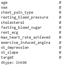
So, there are no missing entries in the dataset that’s great. Next, we will move towards exploring the dataset by performing detailed EDA
Exploratory Data Analysis (EDA)
# first checking the shape of the dataset
dt.shape

So, there is a total of 1189 records and 11 features with 1 target variable. Let’s check the summary of numerical and categorical features.
# summary statistics of numerical columns
dt.describe(include =[np.number])
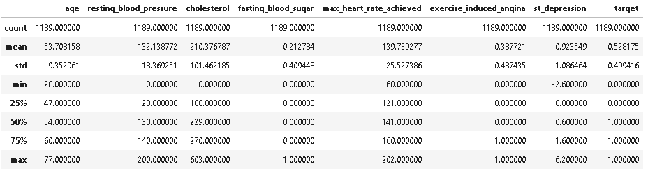
As we can see from the above description resting_blood_pressure and cholesterol have some outliers as they have minimum value of 0 whereas cholesterol has outlier on upper side also having maximum value of 603.
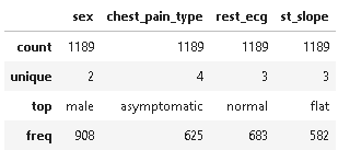
# summary statistics of categorical columns
dt.describe(include =[np.object])
Distribution of target variable
# Plotting attrition of employees
fig, (ax1, ax2) = plt.subplots(nrows=1, ncols=2, sharey=False, figsize=(14,6))

ax1 = dt['target'].value_counts().plot.pie( x="Heart disease" ,y ='no.of patients',
                   autopct = "%1.0f%%",labels=["Heart Disease","Normal"], startangle = 60,ax=ax1);
ax1.set(title = 'Percentage of Heart disease patients in Dataset')

ax2 = dt["target"].value_counts().plot(kind="barh" ,ax =ax2)
for i,j in enumerate(dt["target"].value_counts().values):
    ax2.text(.5,i,j,fontsize=12)
ax2.set(title = 'No. of Heart disease patients in Dataset')
plt.show()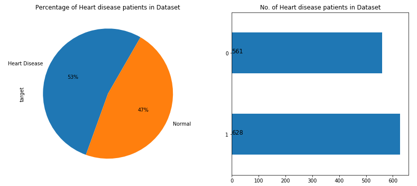
As per the above figure, we can observe that the dataset is balanced having 629 heart disease patients and 561 normal patients.
Distribution of Age and Gender
As we can see from the below pie plot, in this dataset male percentage is way too higher than females whereas the histogram suggests that the average age of the patients in the dataset is around 55.
plt.figure(figsize=(18,12))
plt.subplot(221)
dt["sex"].value_counts().plot.pie(autopct = "%1.0f%%",colors = sns.color_palette("prism",5),startangle = 60,labels=["Male","Female"],
wedgeprops={"linewidth":2,"edgecolor":"k"},explode=[.1,.1],shadow =True)
plt.title("Distribution of Gender")
plt.subplot(222)
ax= sns.distplot(dt['age'], rug=True)
plt.title("Age wise distribution")
plt.show()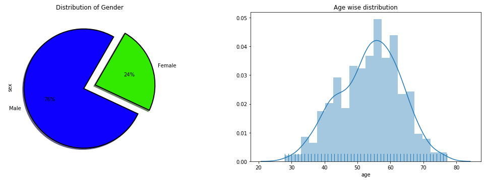
Heart disease-wise distribution of Age and Gender
# creating separate df for normal and heart patients

attr_1=dt[dt['target']==1]

attr_0=dt[dt['target']==0]

# plotting normal patients
fig = plt.figure(figsize=(15,5))
ax1 = plt.subplot2grid((1,2),(0,0))
sns.distplot(attr_0['age'])
plt.title('AGE DISTRIBUTION OF NORMAL PATIENTS', fontsize=15, weight='bold')

ax1 = plt.subplot2grid((1,2),(0,1))
sns.countplot(attr_0['sex'], palette='viridis')
plt.title('GENDER DISTRIBUTION OF NORMAL PATIENTS', fontsize=15, weight='bold' )
plt.show()

#plotting heart patients

fig = plt.figure(figsize=(15,5))
ax1 = plt.subplot2grid((1,2),(0,0))
sns.distplot(attr_1['age'])
plt.title('AGE DISTRIBUTION OF HEART DISEASE PATIENTS', fontsize=15, weight='bold')

ax1 = plt.subplot2grid((1,2),(0,1))
sns.countplot(attr_1['sex'], palette='viridis')
plt.title('GENDER DISTRIBUTION OF HEART DISEASE PATIENTS', fontsize=15, weight='bold' )
plt.show()
From the above plot, we can observe that more male patients account for heart disease in comparison to females whereas mean age for heart disease patients is around 58 to 60 years.
Distribution of Chest Pain Type
# plotting normal patients
fig = plt.figure(figsize=(15,5))
ax1 = plt.subplot2grid((1,2),(0,0))
sns.countplot(attr_0['chest_pain_type'])
plt.title('CHEST PAIN OF NORMAL PATIENTS', fontsize=15, weight='bold')

#plotting heart patients
ax1 = plt.subplot2grid((1,2),(0,1))
sns.countplot(attr_1['chest_pain_type'], palette='viridis')
plt.title('CHEST PAIN OF HEART PATIENTS', fontsize=15, weight='bold' )
plt.show()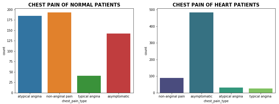
#Exploring the Heart Disease patients based on Chest Pain Type
plot_criteria= ['chest_pain_type', 'target']
cm = sns.light_palette("red", as_cmap=True)
(round(pd.crosstab(dt[plot_criteria[0]], dt[plot_criteria[1]], normalize='columns') * 100,2)).style.background_gradient(cmap = cm)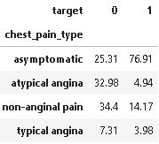
As we can see from the above plot and statistics, 76.91% of the chest pain type of heart disease patients have asymptomatic chest pain.
Asymptomatic heart attacks also known as silent myocardial infarction (SMI) cause around 45-50% of casualties due to cardiac ailments and lead to premature deaths in India.
The symptoms of SMI are very mild in comparison to a regular heart attack; Due to its mild nature, it is also described as a silent killer. The symptoms of SMI are very brief and hence confused with regular discomfort and most often ignored [1].
Distribution of Rest ECG
# plotting normal patients
fig = plt.figure(figsize=(15,5))
ax1 = plt.subplot2grid((1,2),(0,0))
sns.countplot(attr_0['rest_ecg'])
plt.title('REST ECG OF NORMAL PATIENTS', fontsize=15, weight='bold')

#plotting heart patients
ax1 = plt.subplot2grid((1,2),(0,1))
sns.countplot(attr_1['rest_ecg'], palette='viridis')
plt.title('REST ECG OF HEART PATIENTS', fontsize=15, weight='bold' )
plt.show()
#Exploring the Heart Disease patients based on REST ECG
plot_criteria= ['rest_ecg', 'target']
cm = sns.light_palette("red", as_cmap=True)
(round(pd.crosstab(dt[plot_criteria[0]], dt[plot_criteria[1]], normalize='columns') * 100,2)).style.background_gradient(cmap = cm)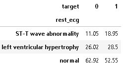
An electrocardiogram (ECG) records the electrical signals of your heart. It’s a common diagnostic test for diagnosing heart problems and monitoring the status of the heart in varied situations. However, ECG also has some of its limitations in detecting heart disease as it measures heart rate and rhythm of the heart but sometimes it doesn’t necessarily show blockages in the arteries and that’s the reason in this dataset around 52% of heart disease patients have normal ECG.
Distribution of ST-Slope
# plotting normal patients
fig = plt.figure(figsize=(15,5))
ax1 = plt.subplot2grid((1,2),(0,0))
sns.countplot(attr_0['st_slope'])
plt.title('ST SLOPE OF NORMAL PATIENTS', fontsize=15, weight='bold')

#plotting heart patients
ax1 = plt.subplot2grid((1,2),(0,1))
sns.countplot(attr_1['st_slope'], palette='viridis')
plt.title('ST SLOPE OF HEART PATIENTS', fontsize=15, weight='bold' )
plt.show()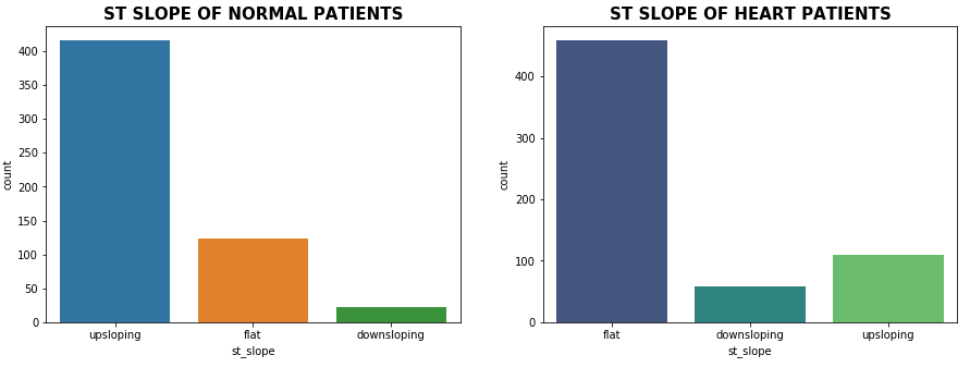
#Exploring the Heart Disease patients based on ST Slope
plot_criteria= ['st_slope', 'target']
cm = sns.light_palette("red", as_cmap=True)
(round(pd.crosstab(dt[plot_criteria[0]], dt[plot_criteria[1]], normalize='columns') * 100,2)).style.background_gradient(cmap = cm)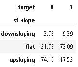
The ST segment /heart rate slope (ST/HR slope), has been proposed as a more accurate ECG criterion for diagnosing significant coronary artery disease (CAD) in most of the research papers.
As we can see from the above plot upsloping is a positive sign as 74% of the normal patients have upslope whereas 72.97% of heart patients have flat sloping.
Distribution of Numerical features
sns.pairplot(dt, hue = 'target', vars = ['age', 'resting_blood_pressure', 'cholesterol'] )
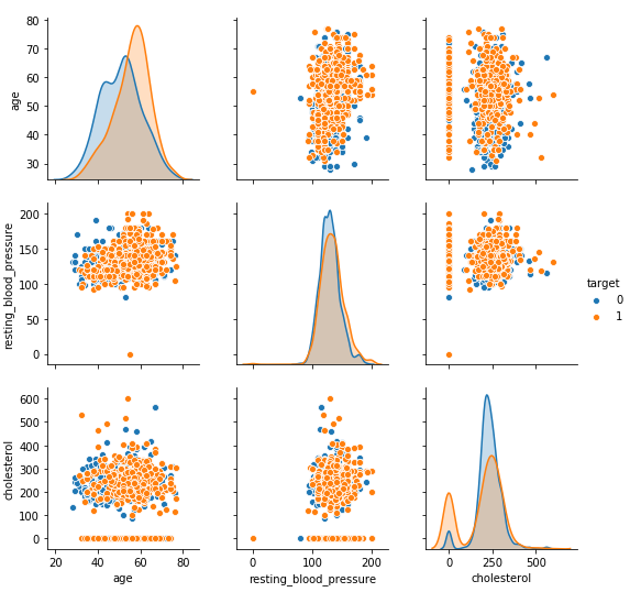
From the above plot, it is clear that as age increases chances of heart disease increases.
Distribution of Cholesterol vs Resting BP
sns.scatterplot(x = 'resting_blood_pressure', y = 'cholesterol', hue = 'target', data = dt)
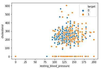
Observation:
From the above plot, we can observe that higher cholesterol with high blood pressure levels results in heart disease whereas normal patients have both cholesterol and blood pressure within the nominal range.
Further, we can see outliers clearly as for some of the patient’s cholesterol is 0 whereas for one patient both cholesterol and resting bp is 0 which may be due to missing entries we will filter these outliers in the next step.
Distribution of Age vs Resting BP
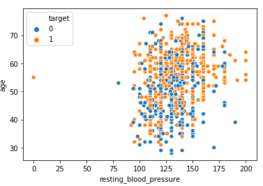
Observation:
From the above scatterplot, we can observe that older patients with higher blood pressure levels >150 are more prone to heart disease in comparison to younger patients <50 years of age.
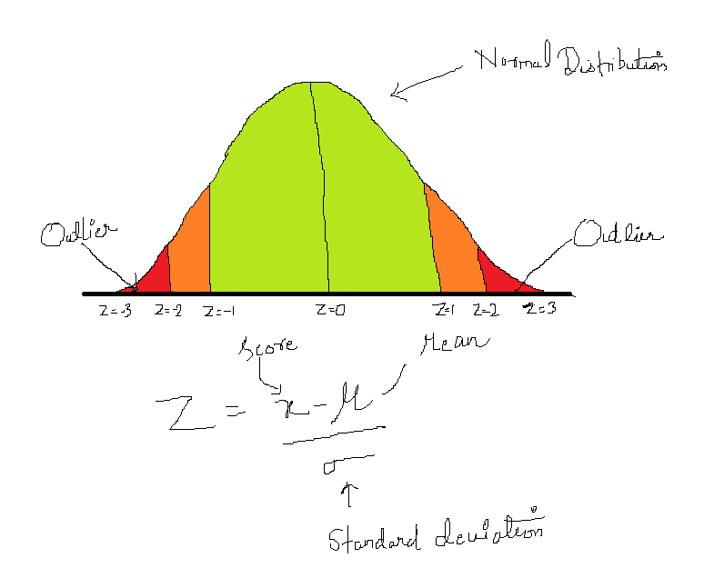
Outlier Detection & Removal
Before detecting outliers, we must know what is an outlier and how it can affect the modeling process. Outlier is defined as a relatively very large or small value in comparison to the rest of the records in the dataset. It may occur due to human errors, changes in system behavior, or instrument error or it may be a genuine data occurred due to natural deviation of the population.
From the EDA we have found that numerical features i.e., age, resting blood pressure, cholesterol, and maximum heart rate achieved has outliers.
# filtering numeric features as age , resting bp, cholestrol and max heart rate achieved has outliers as per EDA

dt_numeric = dt[['age','resting_blood_pressure','cholesterol','max_heart_rate_achieved']]

# calculating zscore of numeric columns in the dataset
z = np.abs(stats.zscore(dt_numeric))
print(z)
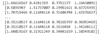
By seeing the above points, it’s very difficult to estimate which points are outliers so we will now define the threshold.
So, in this case, we have defined threshold >3, i.e., points that are falling beyond 3 standard deviations both in case of large and small values will be treated as outliers.
# Defining threshold for filtering outliers
threshold = 3
print(np.where(z > 3))

Here the first array denotes a list of row numbers and the second array respective column numbers, which means z[30][2] has a Z-score higher than 3. There is a total of 17 data points that are outliers.
Filtering outliers
#filtering outliers retaining only those data points which are below threshhold
dt = dt[(z < 3).all(axis=1)]
Now, we can check the shape of the dataset using dt.shape

Great !! all the 17 data points which are outliers are now removed.
Now before splitting the dataset into train and test we first encode categorical variables as dummy variables and segregate feature and the target variable.
## encoding categorical variables
dt = pd.get_dummies(dt, drop_first=True)

dt.head()
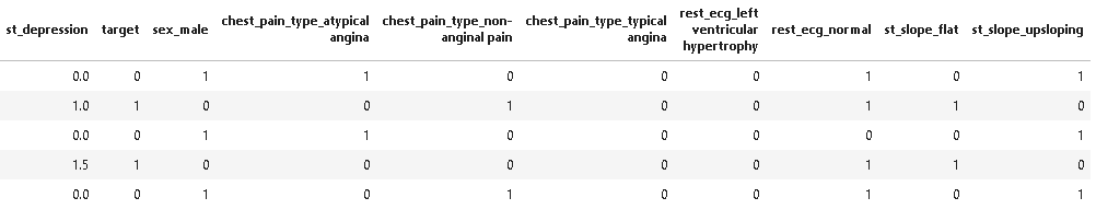
So, after dummy variables we have total of 15 features in the dataset.
Creating Feature and Target variable
# segregating dataset into features i.e., X and target variables i.e., y
X = dt.drop(['target'],axis=1)
y = dt['target']
Checking Correlation
#Correlation with Response Variable class

X.corrwith(y).plot.bar(
        figsize = (16, 4), title = "Correlation with Diabetes", fontsize = 15,
        rot = 90, grid = True)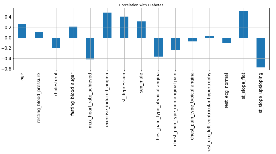
From the above plot, we can observe that excercise_induced_angina, st_slope_flat, st_depression and sex_male are highly positive correlated variables which signify that with an increase in their value chances of heart disease increases.
Train Test Split
We have performed an 80:20 split i.e., 80% of the data will be used for training the machine learning model, and the rest 20% will be used for testing the model.
X_train, X_test, y_train, y_test = train_test_split(X, y, stratify=y, test_size=0.2,shuffle=True, random_state=5)
## checking distribution of traget variable in train test split
print('Distribution of traget variable in training set')
print(y_train.value_counts())
print('Distribution of traget variable in test set')
print(y_test.value_counts())
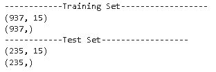
print('------------Training Set------------------')
print(X_train.shape)
print(y_train.shape)
print('------------Test Set------------------')
print(X_test.shape)
print(y_test.shape)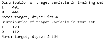
As we can see from the above distribution, the target variable has a balanced distribution in both the training and test set.
Feature Normalization
As we can see in the dataset, many variables have 0,1 values whereas some values have continuous values of different scales which may result in giving higher priority to large-scale values to handle this scenario we have to normalize the features having continuous values in the range of [0,1].
So for normalization, we have used MinMaxScaler for scaling values in the range of [0,1]. Firstly, we have to fit and transform the values on the training set i.e., X_train while for the testing set we have to only transform the values.
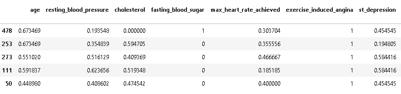
from sklearn.preprocessing import MinMaxScaler
scaler = MinMaxScaler()
X_train[['age','resting_blood_pressure','cholesterol','max_heart_rate_achieved','st_depression']] = scaler.fit_transform(X_train[['age','resting_blood_pressure','cholesterol','max_heart_rate_achieved','st_depression']])
X_train.head()
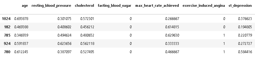
X_test[['age','resting_blood_pressure','cholesterol','max_heart_rate_achieved','st_depression']] = scaler.transform(X_test[['age','resting_blood_pressure','cholesterol','max_heart_rate_achieved','st_depression']])
X_test.head()
Cross-Validation
Next before training and testing machine learning model we will do 10-fold cross-validation to understand which machine learning model is performing well within the training set. So for this step first we have to define the machine learning model and in this project we will be using 13 machine learning algorithms with combinations of different hyperparameters. After defining the machine learning model we will perform 10-fold cross-validation of all the machine learning algorithms.
from sklearn import model_selection
from sklearn.model_selection import cross_val_score
import xgboost as xgb
# function initializing baseline machine learning models
def GetBasedModel():
basedModels = []
basedModels.append(('LR_L2' , LogisticRegression(penalty='l2')))
basedModels.append(('LDA' , LinearDiscriminantAnalysis()))
basedModels.append(('KNN7' , KNeighborsClassifier(7)))
basedModels.append(('KNN5' , KNeighborsClassifier(5)))
basedModels.append(('KNN9' , KNeighborsClassifier(9)))
basedModels.append(('KNN11' , KNeighborsClassifier(11)))
basedModels.append(('CART' , DecisionTreeClassifier()))
basedModels.append(('NB' , GaussianNB()))
basedModels.append(('SVM Linear' , SVC(kernel='linear',gamma='auto',probability=True)))
basedModels.append(('SVM RBF' , SVC(kernel='rbf',gamma='auto',probability=True)))
basedModels.append(('AB' , AdaBoostClassifier()))
basedModels.append(('GBM' , GradientBoostingClassifier(n_estimators=100,max_features='sqrt')))
basedModels.append(('RF_Ent100' , RandomForestClassifier(criterion='entropy',n_estimators=100)))
basedModels.append(('RF_Gini100' , RandomForestClassifier(criterion='gini',n_estimators=100)))
basedModels.append(('ET100' , ExtraTreesClassifier(n_estimators= 100)))
basedModels.append(('ET500' , ExtraTreesClassifier(n_estimators= 500)))
basedModels.append(('MLP', MLPClassifier()))
basedModels.append(('SGD3000', SGDClassifier(max_iter=1000, tol=1e-4)))
basedModels.append(('XGB_2000', xgb.XGBClassifier(n_estimators= 2000)))
basedModels.append(('XGB_500', xgb.XGBClassifier(n_estimators= 500)))
basedModels.append(('XGB_100', xgb.XGBClassifier(n_estimators= 100)))
basedModels.append(('XGB_1000', xgb.XGBClassifier(n_estimators= 1000)))
basedModels.append(('ET1000' , ExtraTreesClassifier(n_estimators= 1000)))
return basedModels
# function for performing 10-fold cross validation of all the baseline models
def BasedLine2(X_train, y_train,models):
# Test options and evaluation metric
num_folds = 10
scoring = 'accuracy'
seed = 7
results = []
names = []
for name, model in models:
kfold = model_selection.KFold(n_splits=10, random_state=seed)
cv_results = model_selection.cross_val_score(model, X_train, y_train, cv=kfold, scoring=scoring)
results.append(cv_results)
names.append(name)
msg = "%s: %f (%f)" % (name, cv_results.mean(), cv_results.std())
print(msg)
return results,msg
models = GetBasedModel()
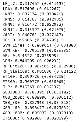
names,results = BasedLine2(X_train, y_train,models)
From the above results, it is clear that the Random forest with criterion entropy and 100 estimators outperformed others by attaining accuracy of 93.49%.
Model building
In this step, we will train all the machine learning models which we have cross-validated in the previous the step we will evaluate all the machine learning models and later compare their performance on test set.
# random forest model with criterion = entropy

rf_ent = RandomForestClassifier(criterion='entropy',n_estimators=100)
rf_ent.fit(X_train, y_train)
y_pred_rfe = rf_ent.predict(X_test)

# multi layer perceptron

mlp = MLPClassifier()
mlp.fit(X_train,y_train)
y_pred_mlp = mlp.predict(X_test)

# K nearest neighbour with n=9

knn = KNeighborsClassifier(9)
knn.fit(X_train,y_train)
y_pred_knn = knn.predict(X_test)

# extra tree classifier with n_estimators=100

et_100 = ExtraTreesClassifier(n_estimators= 100)
et_100.fit(X_train,y_train)
y_pred_et_100 = et_100.predict(X_test)

# XGBoost with n_estimators =500

import xgboost as xgb
xgb = xgb.XGBClassifier(n_estimators= 500)
xgb.fit(X_train,y_train)
y_pred_xgb = xgb.predict(X_test)

# support vector machine with kernel = linear

svc = SVC(kernel='linear',gamma='auto',probability=True)
svc.fit(X_train,y_train)
y_pred_svc = svc.predict(X_test)

# Stochastic Gradient Descent

sgd = SGDClassifier(max_iter=1000, tol=1e-4)
sgd.fit(X_train,y_train)
y_pred_sgd = sgd.predict(X_test)

# Adaboost Classifier

ada = AdaBoostClassifier()
ada.fit(X_train,y_train)
y_pred_ada = ada.predict(X_test)

# Decision Tree (CART)

decc = DecisionTreeClassifier()
decc.fit(X_train,y_train)
y_pred_decc = decc.predict(X_test)

# Gradient Boosting Machine

gbm = GradientBoostingClassifier(n_estimators=100,max_features='sqrt')
gbm.fit(X_train,y_train)
y_pred_gbm = gbm.predict(X_test)
Model Evaluation
In this step, we will evaluate all the 13 machine learning models on the test set and compare their performance. Further, we will select the top 3 best-performed machine learning models.
In this step, we will first define which evaluation metrics we will use to evaluate our model. The most important evaluation metric for this problem domain is sensitivity, specificity, Precision, F1-measure, and ROC AUC curve. Apart from them, we will use two additional performance measures which are more reliable statistical measures i.e., Matthews correlation coefficient (MCC) and Log Loss.
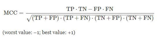
The Matthews correlation coefficient (MCC), is a statistical estimate that produces a high score only if the prediction obtained good results in all of the four confusion matrix categories (true positives, false negatives, true negatives, and false positives), proportionally both to the size of positive elements and the size of negative elements in the dataset.
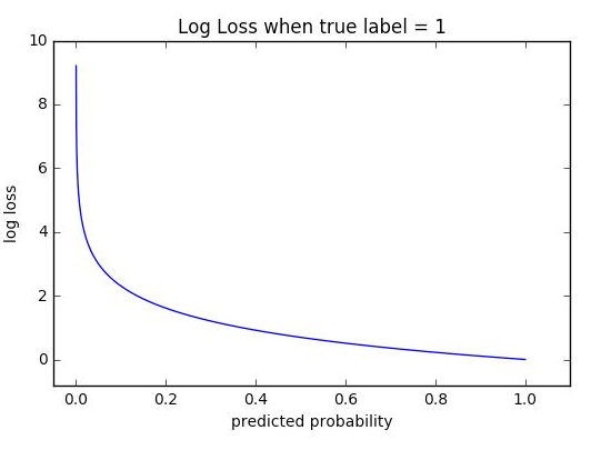
Logarithmic loss measures the performance of a classification model where the prediction input is a probability value between 0 and 1. The goal of our machine learning models is to minimize this value. A perfect model would have a log loss of 0. Log loss increases as the predicted probability diverge from the actual label. So predicting a probability of .012 when the actual observation label is 1 would be bad and result in a high log loss.
The graph below shows the range of possible log loss values given a true observation (isDog = 1). As the predicted probability approaches 1, log loss slowly decreases. As the predicted probability decreases, however, the log loss increases rapidly. Log loss penalizes both types of errors, but especially those predictions that are confident and wrong!
As Random forest model was the best-performed model on cross-validation. So, we will first evaluate a random forest and later compare its performance with other models.
CM=confusion_matrix(y_test,y_pred_rfe)
sns.heatmap(CM, annot=True)

TN = CM[0][0]
FN = CM[1][0]
TP = CM[1][1]
FP = CM[0][1]
specificity = TN/(TN+FP)
loss_log = log_loss(y_test, y_pred_rfe)
acc= accuracy_score(y_test, y_pred_rfe)
roc=roc_auc_score(y_test, y_pred_rfe)
prec = precision_score(y_test, y_pred_rfe)
rec = recall_score(y_test, y_pred_rfe)
f1 = f1_score(y_test, y_pred_rfe)

mathew = matthews_corrcoef(y_test, y_pred_rfe)
model_results =pd.DataFrame([['Random Forest',acc, prec,rec,specificity, f1,roc, loss_log,mathew]],
               columns = ['Model', 'Accuracy','Precision', 'Sensitivity','Specificity', 'F1 Score','ROC','Log_Loss','mathew_corrcoef'])

model_results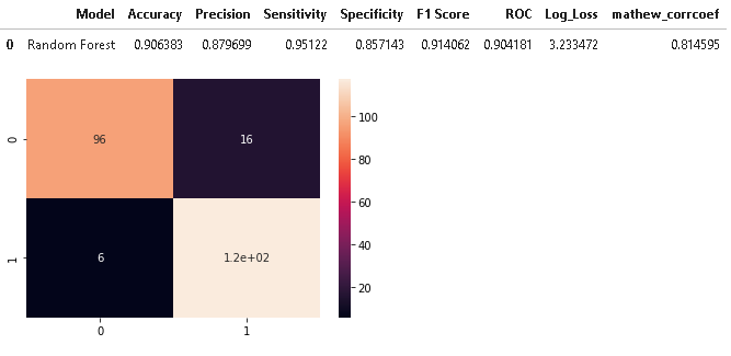
Comparison with other Models
data = {        'MLP': y_pred_mlp,
                'KNN': y_pred_knn,
                'EXtra tree classifier': y_pred_et_100,
                'XGB': y_pred_xgb,
                'SVC': y_pred_svc,
                'SGD': y_pred_sgd,
                'Adaboost': y_pred_ada,
                'CART': y_pred_decc,
                'GBM': y_pred_gbm }

models = pd.DataFrame(data)

for column in models:
    CM=confusion_matrix(y_test,models[column])

    TN = CM[0][0]
    FN = CM[1][0]
    TP = CM[1][1]
    FP = CM[0][1]
    specificity = TN/(TN+FP)
    loss_log = log_loss(y_test, models[column])
    acc= accuracy_score(y_test, models[column])
    roc=roc_auc_score(y_test, models[column])
    prec = precision_score(y_test, models[column])
    rec = recall_score(y_test, models[column])
    f1 = f1_score(y_test, models[column])

    mathew = matthews_corrcoef(y_test, models[column])
    results =pd.DataFrame([[column,acc, prec,rec,specificity, f1,roc, loss_log,mathew]],
               columns = ['Model', 'Accuracy','Precision', 'Sensitivity','Specificity', 'F1 Score','ROC','Log_Loss','mathew_corrcoef'])
    model_results = model_results.append(results, ignore_index = True)

model_results
Findings
As we can see from the above results, XGBoost Classifier is the best performer as it has the highest test accuracy of 0.9191, the sensitivity of 0.943 and specificity of 0.89, and the highest f1-score of 0.9243 and lowest Log Loss of 2.792 whereas Random forest attained the highest sensitivity of 95.122%.
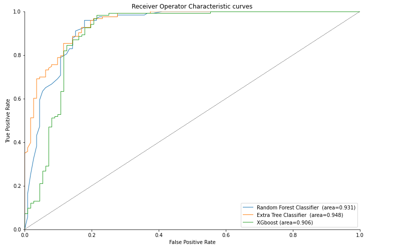
ROC Curve
def roc_auc_plot(y_true, y_proba, label=' ', l='-', lw=1.0):
    from sklearn.metrics import roc_curve, roc_auc_score
    fpr, tpr, _ = roc_curve(y_true, y_proba[:,1])
    ax.plot(fpr, tpr, linestyle=l, linewidth=lw,
            label="%s (area=%.3f)"%(label,roc_auc_score(y_true, y_proba[:,1])))

f, ax = plt.subplots(figsize=(12,8))


roc_auc_plot(y_test,rf_ent.predict_proba(X_test),label='Random Forest Classifier ',l='-')
roc_auc_plot(y_test,et_100.predict_proba(X_test),label='Extra Tree Classifier ',l='-')
roc_auc_plot(y_test,xgb.predict_proba(X_test),label='XGboost',l='-')

ax.plot([0,1], [0,1], color='k', linewidth=0.5, linestyle='--',
        )
ax.legend(loc="lower right")
ax.set_xlabel('False Positive Rate')
ax.set_ylabel('True Positive Rate')
ax.set_xlim([0, 1])
ax.set_ylim([0, 1])
ax.set_title('Receiver Operator Characteristic curves')
sns.despine()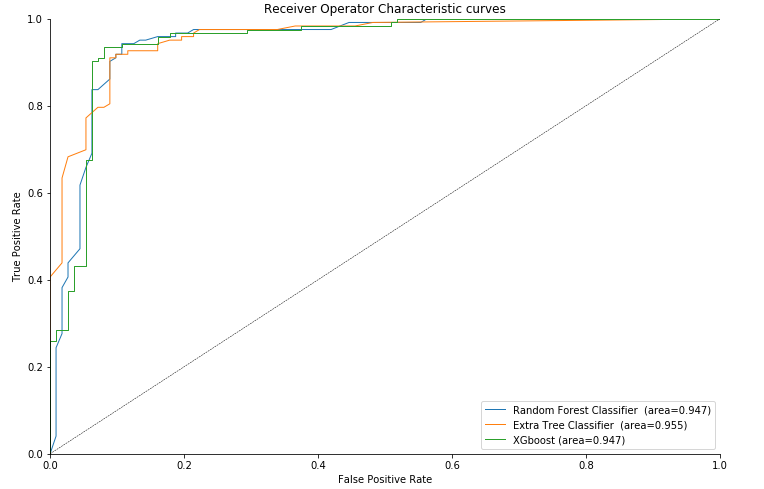
As we can see the highest average area under the curve (AUC) of 0.950 is attained by Extra Tree Classifier.
Feature Selection
Feature selection (FS) is the method for filtering out irrelevant or redundant features from the dataset, which helps the machine learning model in reducing training time, building simple models, and interpreting features.
In this project, we have used two filter-based FS techniques: Pearson Correlation Coefficient and Chi-square, one wrapper-based FS: Recursive Feature Elimination, and three embedded FS methods: embedded logistic regression, embedded random forest, and embedded Light GBM. After applying all these FS methods we have selected only those features which are voted by a majority of FS methods: i.e., voted by at least 5 out of 6 FS methods.
#Pearson correlation FS method

num_feats=11
def cor_selector(X, y,num_feats):
    cor_list = []
    feature_name = X.columns.tolist()
    # calculate the correlation with y for each feature
    for i in X.columns.tolist():
        cor = np.corrcoef(X[i], y)[0, 1]
        cor_list.append(cor)
    # replace NaN with 0
    cor_list = [0 if np.isnan(i) else i for i in cor_list]
    # feature name
    cor_feature = X.iloc[:,np.argsort(np.abs(cor_list))[-num_feats:]].columns.tolist()
    # feature selection? 0 for not select, 1 for select
    cor_support = [True if i in cor_feature else False for i in feature_name]
    return cor_support, cor_feature
cor_support, cor_feature = cor_selector(X, y,num_feats)

# Chi-square

from sklearn.feature_selection import SelectKBest
from sklearn.feature_selection import chi2
from sklearn.preprocessing import MinMaxScaler
X_norm = MinMaxScaler().fit_transform(X)
chi_selector = SelectKBest(chi2, k=num_feats)
chi_selector.fit(X_norm, y)
chi_support = chi_selector.get_support()
chi_feature = X.loc[:,chi_support].columns.tolist()

# Recursive Feature elimination
from sklearn.feature_selection import RFE

rfe_selector = RFE(estimator=LogisticRegression(), n_features_to_select=num_feats, step=10, verbose=5)
rfe_selector.fit(X_norm, y)
rfe_support = rfe_selector.get_support()
rfe_feature = X.loc[:,rfe_support].columns.tolist()

# Embedded Logistic Regression

embeded_lr_selector = SelectFromModel(LogisticRegression(penalty="l2", solver='lbfgs'), max_features=num_feats)
embeded_lr_selector.fit(X_norm, y)

embeded_lr_support = embeded_lr_selector.get_support()
embeded_lr_feature = X.loc[:,embeded_lr_support].columns.tolist()

# Embedded Random forest

embeded_rf_selector = SelectFromModel(RandomForestClassifier(n_estimators=100, criterion='gini'), max_features=num_feats)
embeded_rf_selector.fit(X, y)

embeded_rf_support = embeded_rf_selector.get_support()
embeded_rf_feature = X.loc[:,embeded_rf_support].columns.tolist()


# embedded light gbm

from lightgbm import LGBMClassifier

lgbc=LGBMClassifier(n_estimators=500, learning_rate=0.05, num_leaves=32, colsample_bytree=0.2,
            reg_alpha=3, reg_lambda=1, min_split_gain=0.01, min_child_weight=40)

embeded_lgb_selector = SelectFromModel(lgbc, max_features=num_feats)
embeded_lgb_selector.fit(X, y)

embeded_lgb_support = embeded_lgb_selector.get_support()
embeded_lgb_feature = X.loc[:,embeded_lgb_support].columns.tolist()

# put all selection together

feature_name = X.columns
feature_selection_df = pd.DataFrame({'Feature':feature_name, 'Pearson':cor_support, 'Chi-2':chi_support, 'RFE':rfe_support, 'Logistics':embeded_lr_support,
                                    'Random Forest':embeded_rf_support, 'LightGBM':embeded_lgb_support})
# count the selected times for each feature
feature_selection_df['Total'] = np.sum(feature_selection_df, axis=1)
# display the top 100
feature_selection_df = feature_selection_df.sort_values(['Total','Feature'] , ascending=False)
feature_selection_df.index = range(1, len(feature_selection_df)+1)
feature_selection_df.head(num_feats)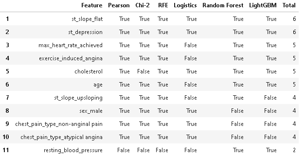
As we can observe from the above results, there are only 11 features that are selected by at least one FS method. The features: fasting_blood_sugar, chest_pain_type_typical angina, rest_ecg_left ventricular hypertrophy, and rest_ecg_normal are missing in the table because they are not considered important features by any of the FS methods.
So, now we will only select the top 6 features which are voted by 5 out of 6 FS methods i.e., st_slope_flat, st_depression, max_heart_rate_achieved, exercise_induced_angina, cholesterol, and age. Further, we will retrain the machine learning models with 6 selected features and compare their performance to check if there will be any performance drop post feature selection.
# segregating dataset into features i.e., X and target variables i.e., y
X = X.drop(['st_slope_upsloping','fasting_blood_sugar','resting_blood_pressure','sex_male','chest_pain_type_typical angina','chest_pain_type_non-anginal pain','chest_pain_type_atypical angina','rest_ecg_left ventricular hypertrophy','rest_ecg_normal'],axis=1)
y = dt['target']

# train test split
X_train, X_test, y_train, y_test = train_test_split(X, y, stratify=y, test_size=0.2,shuffle=True, random_state=5)

# feature normalization
scaler = MinMaxScaler()
X_train[['age','cholesterol','max_heart_rate_achieved','st_depression']] = scaler.fit_transform(X_train[['age','cholesterol','max_heart_rate_achieved','st_depression']])
X_test[['age','cholesterol','max_heart_rate_achieved','st_depression']] = scaler.transform(X_test[['age','cholesterol','max_heart_rate_achieved','st_depression']])

# cross-validation of models
models = GetBasedModel()
names,results = BasedLine2(X_train, y_train,models)
Model Evaluation
Now, we have to evaluate all the machine learning algorithms after feature selection i.e., with six features.
As random forest attained the highest 10-fold cross-validation accuracy post feature selection, we will assign it as a base model and evaluate it first later comparing its performance with other machine learning algorithms.
# fitting random forest model
rf_ent = RandomForestClassifier(criterion='entropy',n_estimators=100)
rf_ent.fit(X_train, y_train)
y_pred_rfe = rf_ent.predict(X_test)

#model evaluation
CM=confusion_matrix(y_test,y_pred_rfe)
sns.heatmap(CM, annot=True)

TN = CM[0][0]
FN = CM[1][0]
TP = CM[1][1]
FP = CM[0][1]
specificity = TN/(TN+FP)
loss_log = log_loss(y_test, y_pred_rfe)
acc= accuracy_score(y_test, y_pred_rfe)
roc=roc_auc_score(y_test, y_pred_rfe)
prec = precision_score(y_test, y_pred_rfe)
rec = recall_score(y_test, y_pred_rfe)
f1 = f1_score(y_test, y_pred_rfe)

mathew = matthews_corrcoef(y_test, y_pred_rfe)
model_results =pd.DataFrame([['Random Forest',acc, prec,rec,specificity, f1,roc, loss_log,mathew]],
               columns = ['Model', 'Accuracy','Precision', 'Sensitivity','Specificity', 'F1 Score','ROC','Log_Loss','mathew_corrcoef'])

model_results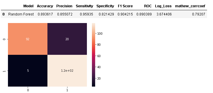
# multi layer perceptron

mlp = MLPClassifier()
mlp.fit(X_train,y_train)
y_pred_mlp = mlp.predict(X_test)

# K nearest neighbour with n=9

knn = KNeighborsClassifier(9)
knn.fit(X_train,y_train)
y_pred_knn = knn.predict(X_test)

# extra tree classifier with n_estimators=100

et_100 = ExtraTreesClassifier(n_estimators= 100)
et_100.fit(X_train,y_train)
y_pred_et_100 = et_100.predict(X_test)

# XGBoost with n_estimators =500

import xgboost as xgb
xgb = xgb.XGBClassifier(n_estimators= 500)
xgb.fit(X_train,y_train)
y_pred_xgb = xgb.predict(X_test)

# support vector machine with kernel = linear

svc = SVC(kernel='linear',gamma='auto',probability=True)
svc.fit(X_train,y_train)
y_pred_svc = svc.predict(X_test)

# Stochastic Gradient Descent

sgd = SGDClassifier(max_iter=1000, tol=1e-4)
sgd.fit(X_train,y_train)
y_pred_sgd = sgd.predict(X_test)

# Adaboost Classifier

ada = AdaBoostClassifier()
ada.fit(X_train,y_train)
y_pred_ada = ada.predict(X_test)

# Decision Tree (CART)

decc = DecisionTreeClassifier()
decc.fit(X_train,y_train)
y_pred_decc = decc.predict(X_test)

# Gradient Boosting Machine

gbm = GradientBoostingClassifier(n_estimators=100,max_features='sqrt')
gbm.fit(X_train,y_train)
y_pred_gbm = gbm.predict(X_test)

# model evaluation

data = {

                'MLP2': y_pred_mlp,
                'KNN2': y_pred_knn,
                'EXtra tree classifier': y_pred_et1000,
                'XGB2': y_pred_xgb,
                'SVC2': y_pred_svc,
                'SGD2': y_pred_sgd,
                'Adaboost': y_pred_ada,
                'CART': y_pred_decc,
                'GBM': y_pred_gbm }

models = pd.DataFrame(data)

for column in models:
    CM=confusion_matrix(y_test,models[column])

    TN = CM[0][0]
    FN = CM[1][0]
    TP = CM[1][1]
    FP = CM[0][1]
    specificity = TN/(TN+FP)
    loss_log = log_loss(y_test, models[column])
    acc= accuracy_score(y_test, models[column])
    roc=roc_auc_score(y_test, models[column])
    prec = precision_score(y_test, models[column])
    rec = recall_score(y_test, models[column])
    f1 = f1_score(y_test, models[column])

    mathew = matthews_corrcoef(y_test, models[column])
    results =pd.DataFrame([[column,acc, prec,rec,specificity, f1,roc, loss_log,mathew]],
               columns = ['Model', 'Accuracy','Precision', 'Sensitivity','Specificity', 'F1 Score','ROC','Log_Loss','mathew_corrcoef'])
    model_results = model_results.append(results, ignore_index = True)

model_results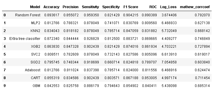
Plotting ROC Plot
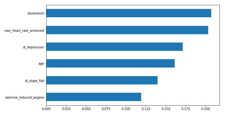
Feature Importance
In this step, we will plot important features of the random forest model which are highly contributing to predicting heart disease.
feat_importances = pd.Series(rf_ent.feature_importances_, index=X_train.columns)
feat_importances.sort_values().plot(kind="barh",figsize=(10, 6))
Conclusion
- In this article, we have analyzed the Heart Disease Dataset (Comprehensive) and performed detailed data analysis and data processing.
- Trained and evaluated 10 machine learning models and compared their performance and found that the Random forest model with entropy criterion outperformed others with an accuracy of 90.63%.
- Further, we have performed a majority vote feature selection technique comprising two filters based, one wrapper based, and 3 embedded feature selection methods.
- After feature selection, Random Forest remains the best performing algorithm having an accuracy of 89.36% i.e., less than 1% drop before feature selection.
- We have also plotted the feature importance plot and found that the top 3 most contributing features were Cholesterol, Max heart rate achieved, and st_depression.
We have also uploaded a detailed video on heart disease prediction on our youtube channel WisdomML. Feel free to check this out also.
Thank you for reading! Feel free to share your thoughts and ideas.