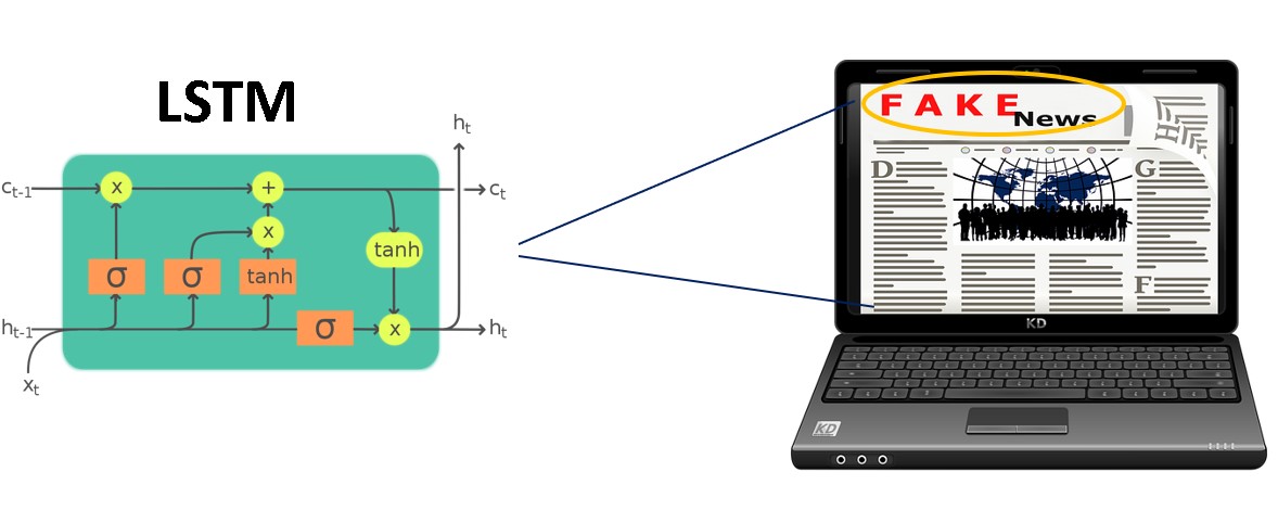
In this article, we will demonstrate the application of the deep learning technique i.e., Long Short-Term Memory (LSTM) for the detection of fake news by analyzing news article text with news headlines. 

Problem statement

In the last few years, due to the widespread usage of online social networks, fake news spreading at an alarming rate for various commercial and political purposes which is a matter of concern as it has numerous psychological effects on offline society. According to Gartner Research

By 2022, most people in mature economies will consume more false information than true information.

For enterprises, this accelerated rate of fake news content on social media presents a challenging task to not only monitor closely what is being said about their brands directly but also in what contexts, because fake news will directly affect their brand value.

So, in this post, we will discuss how we can detect fake news accurately by analyzing news articles.

About Data

The data used in this case study is the ISOT Fake News Dataset. The dataset contains two types of articles fake and real news. This dataset was collected from real-world sources; the truthful articles were obtained by crawling articles from Reuters.com (a news website). As for the fake news articles, they were collected from unreliable websites that were flagged by Politifact (a fact-checking organization in the USA) and Wikipedia. The dataset contains different types of articles on different topics, however, the majority of articles focused on political and World news topics.

The dataset consists of two CSV files. The first file named True.csv contains more than 12,600 articles from Reuters.com. The second file named Fake.csv contains more than 12,600 articles from different fake news outlet resources. Each article contains the following information:

• article title (News Headline),
• text (News Body),
• subject
• date

The total records in the dataset consist of 44898 records out of which 21417 are true news and 23481 are fake news.

So, next, we will be discussing data pre-processing and data preparation steps required for building Long Term Short Memory (LSTM) model using the Keras library in python. The detailed architecture and mathematics behind LSTM can be found here.

Data processing

In this step, we will read both the datasets (Fake.csv, True.csv) perform some data cleaning, merge both the datasets and shuffle the final dataset.

The code for data processing is shown below:

import numpy as np
import pandas as pd
from collections import defaultdict
import re


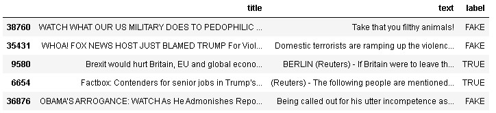
df_fake = pd.read_csv('fake_news_dataset/Fake.csv')
df_fake.head()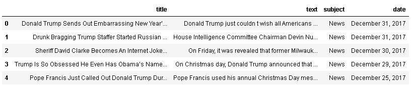

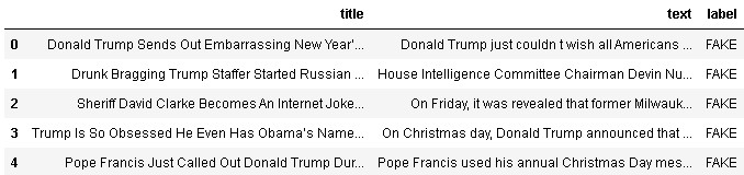
As we only need title and text, so we will drop extra features i.e., subject and date.

# dropping unneccesary features
df_fake=df_fake.drop(['subject','date'],axis=1)

# assigning label 'FAKE' by creating target column i.e., label
df_fake['label'] ='FAKE' 

df_fake.head()

Similarly, we will be processing the True dataset and further merging it with the df_fake data frame to create the final dataset. The code for the same is given below:

df_true = pd.read_csv('fake_news_dataset/True.csv')
df_true=df_true.drop(['subject','date'],axis=1)
df_true['label']='TRUE'

df= pd.concat([df_true, df_fake], ignore_index=True)
df.head()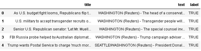

So, we have merged the dataset, but the dataset has a defined sequence of True and Fake labels. So, therefore we need to shuffle the dataset to introduce a randomness in the dataset.

#shuffling the dataset
df=df.reindex(np.random.permutation(df.index))
df.head()

From the dataset, we can observe that True news text contains the source of the news also i.e., 3rd row of True News text starts from BERLIN (Reuters) –, whereas 4th row of True News text starts from (Reuters) –

So, we have to clean the True News text as it affects the model building process as it’s not an important feature for building a fake news detection model.

Therefore, we have to write look ahead regular expression to retain only the text followed by “(Reuters) –“. The code for regular expression-based extraction is shared below:

import re
# function for extracting desired text using regex
def extract_txt(text):
    regex = re.search(r"(?<=\(Reuters\)\s\-\s).*",text)
    if regex:
        return regex.group(0)
    return text
#applying regex function to retain only relevant text
df['text_processed'] = df['text'].apply(extract_txt)

#checking dataframe containing only True News
df[df.label=="TRUE"]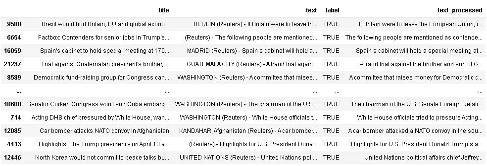

So, as we can see from the above dataset, the text with the True label is cleaned now. Next, we will be using this combined dataset for building the LSTM model.

Data preparation & cleaning

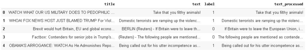
Firstly we will convert the target variable label into binary variable 0 for True news and 1 for Fake news.

# drop extra column
df = df.drop(['text'],axis=1)
df["label"] = df.label.apply(lambda  x:0 if x=='TRUE' else 1)
df.head()

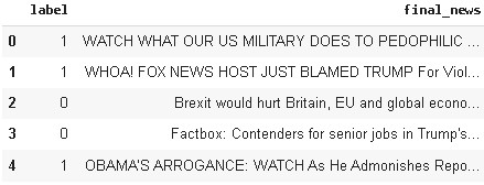
As we have to analyze the whole news article so we have to combine both title and text_processed features. Further, we have to drop unnecessary features i.e., title, text, and text_processed features from the dataset as we have to use only the final combined news column for building the model.

#combining text_processed and title for creating full news article with headline
df['final_news'] = df['title'] + " " + df['text_processed']

# now we can delete extra columns 
cols_del =['title','text','text_processed']
df = df.drop(cols_del,axis=1)

df.head()

In the next step, lowercase the data, although it is commonly overlooked, it is one of the most effective techniques when the data is small. Although the word ‘Good’, ‘good’ and ‘GOOD’ are the same but the neural net model will assign different weights to it resulting in abrupt output which will affect the overall performance of the model.

Further, we will remove the stopwords and all non-alphabetic characters from the dataset. The code for the above-mentioned task is shared below:

#creating list of possible stopwords from nltk library
stop = stopwords.words('english')

def cleanText(txt):
  # lowercaing
    txt = txt.lower()
  # removing stopwords
    txt = ' '.join([word for word in txt.split() if word not in (stop)])
  # removing non-alphabetic characters
    txt = re.sub('[^a-z]',' ',txt)
    return txt  

#applying text cleaning function to clean final_news
df['final_news'] = df['final_news'].apply(cleanText)
df.head()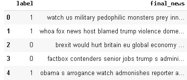

Building Word Embeddings (GLOVE)

In this case study, we will use Global vectors for word representation (GLOVE) word embeddings. It is an unsupervised learning algorithm for obtaining vector representations for words.

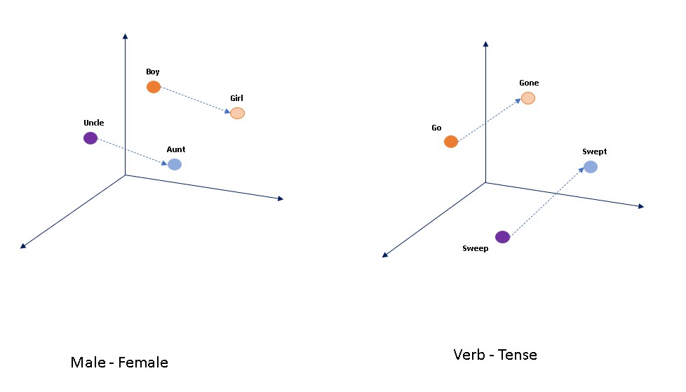
The main idea behind word embedding is that it helps in establishing a contextual representation of words in a document, semantic and syntactic similarity and relationships among different words, etc.

The word embedding is proved to work well with LSTM in the text classification tasks as the model becomes more understandable in terms of contextual knowledge in comparison to only vectorization methods. The visual representation of word embeddings is shown below:

So, now we will set the file path of the Glove embeddings file and will do configuration settings as shown in the code snippet below. For downloading the Glove embedding file you can visit the nlp stanford website.

path = '/content/drive/MyDrive'

EMBEDDING_FILE=f'{path}/glove.6B.50d.txt'

# configuration setting
MAX_SEQUENCE_LENGTH = 100
MAX_VOCAB_SIZE = 20000
EMBEDDING_DIM = 50
VALIDATION_SPLIT = 0.2
BATCH_SIZE = 32
EPOCHS = 10


# creating feature and target variable
X = df.drop(['label'],axis=1)
y = df['label'].values

As we can see from the above code, we have used a maximum sequence length of 100, a maximum vocab size of 20000 (we can experiment to increase it to 25000 or more for better accuracy but it will increase the training time), number of dimensions in this embedding is 50 i.e., each word has 50 dimensions in vector space again we can experiment with 100 dimensions to check for accuracy improvement, validation split of 0.2 will be used means 20% of the training data used for validating the model during the training phase. The batch size used here is 32, we can also experiment with different batch sizes. For the demo purpose, we have used only 10 epochs to train the LSTM model, we can also increase to higher epochs for better results.

Next, we will load the pre-trained word vectors from the embedding file.

Tokenize Text

Next, we will convert sentences (texts) into integers as we know any machine learning or deep learning model doesn’t understand textual data so we have to convert it into number representation.

# load in pre-trained word vectors
print('Loading word vectors...')
word2vec = {}
with open(EMBEDDING_FILE) as f:
  # is just a space-separated text file in the format:
  # word vec[0] vec[1] vec[2] ...
  for line in f:
    values = line.split()
    word = values[0]
    vec = np.asarray(values[1:], dtype='float32')
    word2vec[word] = vec

# convert the sentences (strings) into integers
tokenizer = Tokenizer(num_words=MAX_VOCAB_SIZE)
tokenizer.fit_on_texts(list(X['final_news']))
X = tokenizer.texts_to_sequences(list(X['final_news']))

# pad sequences so that we get a N x T matrix
X = pad_sequences(X, maxlen=MAX_SEQUENCE_LENGTH)
print('Shape of data tensor:', X.shape)

Now, let’s understand the code snippet shown above. First, we have tokenized the final_news text using a tokenizer with a number of words equivalent to the maximum vocab size we have set earlier i.e., 20000. Now, the question comes what is the use of the tokenizer.fit_on_texts and then tokenizer.text_to_sequences.

So, the tokenizer.fit_on_texts is used to create a vocabulary index based on its frequency as it creates the vocabulary index based on word frequency.

For example, if you had the sentences “My skill is different from other students”, “I am a good student”, then word_index[“skill”] = 0, word_index[“student”] = 1 (student appears 2 times, skill appears 1 time), while tokenizer.text_to_sequences basically assign each text in a sentence into a sequence of integers. 

So what it does is that it takes each word in the sentence and replaces it with its corresponding integer value from word_index.

Sequence Padding

Next, we have padded the sequence to the max length of 100 which we declared earlier. This is done to ensure that all the sequences are of the same length as is needed in the case of building a neural network.

Therefore, sequences which are shorter than the max length of 100 are padded with zeroes while longer sequences are truncated to a max length of 100.

Now we have assigned this sequence padded matrix as our feature vector X and our target variable y is label i.e., df[‘label’].

After printing the shape of the tensor we get the matrix shape as 44898 x 100.

Then we have saved the word to id (integers) mapping obtained from the tokenizer into a new variable named word2idx as shown below.

# get word -> integer mapping
word2idx = tokenizer.word_index
print('Found %s unique tokens.' % len(word2idx))

Preparation of Embedding Matrix

After printing the length we found a total of 29101 unique tokens. The next task is to create an embedding matrix. The code for preparing the embedding matrix is shared below.

# prepare embedding matrix
print('Filling pre-trained embeddings...')
num_words = min(MAX_VOCAB_SIZE, len(word2idx) + 1)
embedding_matrix = np.zeros((num_words, EMBEDDING_DIM))
for word, i in word2idx.items():
  if i < MAX_VOCAB_SIZE:
    embedding_vector = word2vec.get(word)
    if embedding_vector is not None:
      # words not found in embedding index will be all zeros.
      embedding_matrix[i] = embedding_vector

As per the code num_words are the minimum of Max_VOCAB_SIZE and length of word2idx+1.

We know MAX_VOCAB_SIZE = 20000 and length of word2idx = 29101. So the number of words is the minimum of these two i.e., 20000.

Next, an embedding matrix is created with the dimension of 50 and 20000 words. The words which will not be found in the matrix will be assigned as zeroes.

Creation of Embedding Layer

Next, we will create an embedding layer that will be used as input in the LSTM model.

# load pre-trained word embeddings into an Embedding layer
# note that we set trainable = False so as to keep the embeddings fixed
embedding_layer = Embedding(
  num_words,
  EMBEDDING_DIM,
  weights=[embedding_matrix],
  input_length=MAX_SEQUENCE_LENGTH,
  trainable=False
)

Model Building

In this step, we will build the deep learning model Long Term Short Memory (LSTM). For this case study, we will be using bi-directional LSTM.

# create an LSTM network with a single LSTM
input_ = Input(shape=(MAX_SEQUENCE_LENGTH,))
x = embedding_layer(input_)
# x = LSTM(15, return_sequences=True)(x)
x = Bidirectional(LSTM(15, return_sequences=True))(x)
x = GlobalMaxPool1D()(x)
output = Dense(1, activation="sigmoid")(x)

model = Model(input_, output)
model.compile(
  loss='binary_crossentropy',
  optimizer='adam',
  metrics=['accuracy']
)
model.summary()

As we can see from the above code, we have used one hidden layer of the Bidirectional LSTM layer of 15 neurons. For accessing the hidden state output for each input time step we have to set return_sequences=”True”. This is also a hyper-parameter that we can experiment with.

Further, we can also experiment with other variants of LSTMs like unidirectional LSTM and GRU. The number of neurons can also be increased to check for performance improvements. The detailed model summary is shown below.

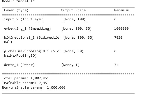
Model Parameters

Here, the main thing to notice is that the total number of model parameters is 1,007,951 whereas training parameters are only 7951 which is the sum of parameters of bidirectional LSTM i.e., 7920 and dense layers parameter i.e., 31. The reason for this is that we have already set trainable = false in case of embedding layer due to which 1000000 parameters of embedding layers left non-trainable.

Train test split

Now we split the feature and target variable into train and test sets in the ratio of 80:20, where 80% of the data is used for training the model and 20% is used for testing.

# train Test split in the ratio of 80:20
X_train, X_test, y_train, y_test = train_test_split(X, y,test_size=0.20,stratify=y, random_state=0)

Fitting model

In this step, we actually fit the model on the training set with batch size =32 and a validation split of 20%

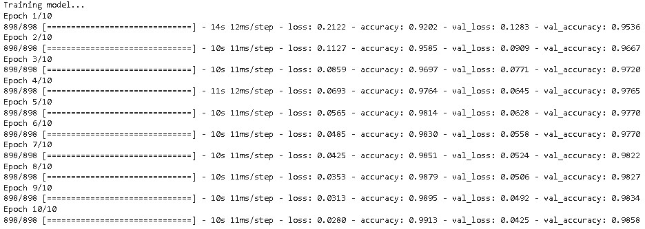
As we can observe from the above result, the model achieved a validation accuracy of 98.58% in just 10 epochs.

The training and validation loss and accuracy plots are shown below to show the progress of model training.

acc = r.history['accuracy']
val_acc = r.history['val_accuracy']
loss = r.history['loss']
val_loss = r.history['val_loss']
epochs_range = range(1, len(r.epoch) + 1)

plt.figure(figsize=(15,5))

plt.subplot(1, 2, 1)
plt.plot(epochs_range, acc, label='Train Set')
plt.plot(epochs_range, val_acc, label='Val Set')
plt.legend(loc="best")
plt.xlabel('Epochs')
plt.ylabel('Accuracy')
plt.title('LSTM Model Accuracy')

plt.subplot(1, 2, 2)
plt.plot(epochs_range, loss, label='Train Set')
plt.plot(epochs_range, val_loss, label='Val Set')
plt.legend(loc="best")
plt.xlabel('Epochs')
plt.ylabel('Loss')
plt.title('LSTM Model Loss')

plt.tight_layout()
plt.show()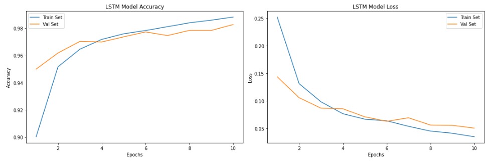

As we can see from the above plot, the model’s validation accuracy reached to 98% at around the 10th epoch.

Model result

The training and test accuracy of the model is shown below.

The confusion matrix of the model is shown below.

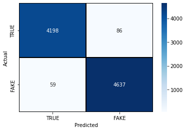
As we can see from the above confusion matrix, the model has shown impressive performance. Now, let’s see the classification report to understand the overall performance from the statistical point of view.

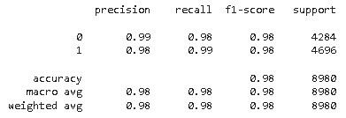
As per the result, our model has a higher recall and F1 score of 99% and 98% for fake news respectively whereas precision is higher for Real news. The better estimate to judge any machine learning or deep learning model performance is the F1-score as it is the harmonic mean of precision and recall.

A higher F1 score of 98% is a fairly good score but we can improve the model performance by tuning its hyper-parameters.

Apart from that, there is one more performance metric that is widely used in binary classification tasks is the Receiver Operating Characteristics curve also known as the ROC curve. The ROC curve of the model is plotted below.

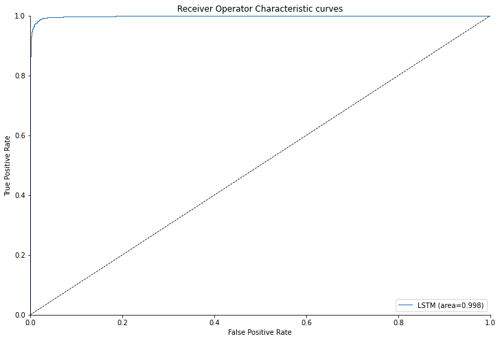
As per the ROC plot above it is evident that the model performs fairly well with a higher Area Under Curve (AUC) of 0.998. AUC of 1 means ideal model.

Model Prediction

This is the most important part of this project i.e., actually using the model to detect fake and real news from sample news articles. But for that, we have to perform certain preprocessing of sample text before feeding them into the LSTM model.

testSent =["Trey Gowdy destroys this clueless DHS employee when asking about the due process of getting on the terror watch list. Her response is priceless:  I m sorry, um, there s not a process afforded the citizen prior to getting on the list.  ",
       "Poland s new prime minister faces a difficult balancing act trying to repair bruised relations with the European Union without alienating the eurosceptic government s core voters. A Western-educated former banker who is fluent in German and English and was sworn in on Monday, Mateusz Morawiecki boasts the credentials needed to negotiate with Brussels. But any compromises to improve relations with Brussels, which sees the ruling Law and Justice (PiS) party as a threat to democracy, would risk upsetting the traditional, Catholic supporters who propelled it into power two years ago. It is a gamble that could backfire, and it is not yet clear how far Morawiecki, 49, and his party, dominated by former Prime Minister Jaroslaw Kaczynski, are ready to go to please Brussels.   The idea to build up international credibility seems rational,  said Jaroslaw Flis, a sociologist at the Jagiellonian University.  But such actions would have to be in complete contrast with what Mateusz Morawiecki would have to do domestically to prevent the PiS from falling apart."
      ]

def predict_text(lst_text):
    test = tokenizer.texts_to_sequences(testSent)
    # pad sequences so that we get a N x T matrix
    testX = pad_sequences(test, maxlen=MAX_SEQUENCE_LENGTH)
    prediction = model.predict(testX)
    df_test = pd.DataFrame(testSent, columns = ['test_sent'])

    df_test['prediction']=prediction
    df_test["test_sent"] = df_test["test_sent"].apply(cleanText)
    df_test['prediction']=df_test['prediction'].apply(lambda x: "Fake" if x>=0.5 else "Real")
    return df_test

#getting the prediction by passing list of sample news articles
df_testsent = predict_text(testSent)
df_testsent

The full code demonstrated in this post is available in this repo.

Conclusion

In this article, we have demonstrated the application of the deep learning model LSTM for the detection of fake news from news articles and it showed outstanding results. Further, we can utilize this model for verifying the genuineness of the online news article generally cropped up on social media websites by integrating this model in the form of a Google Chrome extension or separate web application.

we hope this article will help you in understanding the implementation of the LSTM model for the text classification task.

Thank you for reading! Feel free to share your thoughts and ideas.